Strange Attractor

Introduction

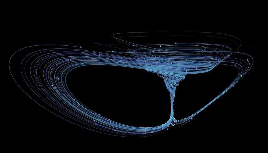
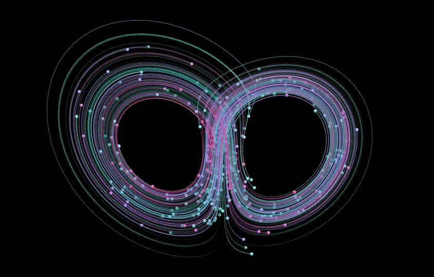
Strange Attractors transform chaotic differential equations into elegant visual art. By simulating the trajectories of particles driven by mathematical rules in three-dimensional space, you can create complex organic structures that reveal "chaotic shapes" — from the butterfly-like Lorenz attractor to the spiraling Aizawa attractor, each equation combination embodies profound mathematical beauty.

Core Capabilities:

• Math-Driven Art: Visualize classic chaotic systems (such as Lorenz, Rössler, Aizawa, etc.) or write custom differential equations
• Dual Rendering Modes: CPU mode supports high-quality trail rendering, GPU mode supports massive particle cloud rendering
• Intelligent Parameter Randomization: Sensitivity-guided local search algorithm to explore stable and visually meaningful parameter combinations with one click
• Full Animation Support: Integrated timeline system with camera movement and parameter animation
• Professional Palette System: Supports Manual, Cosine, and Curve gradient modes, with JSON palettes for rich color expression

---

Mathematical Background

What is a Strange Attractor?

A strange attractor is a special set in a dynamical system with the following characteristics:

• Attractivity: Trajectories in the system are "attracted" to a specific region — regardless of initial position, particles eventually fall into this region
• Strangeness: Trajectories within the region exhibit chaotic, non-periodic complex behavior — seemingly random, yet driven by deterministic equations
• Fractal Structure: Infinitely complex geometric structures unfold within a finite space — zooming in always reveals new details

Intuitive Understanding: Imagine a funnel where water drops fall from different positions but eventually converge at the bottom — this is "attractivity." However, the "funnel" of a strange attractor is not a simple cone, but a complex surface with infinite folds, and the paths of water drops through it never exactly repeat — this is "strangeness."

Differential Equation Systems

Strange attractors are defined by systems of ordinary differential equations (ODEs):

where are functions defining the velocity field. The system computes particle trajectories step by step through numerical integration.

Intuitive Understanding: Imagine a particle floating in three-dimensional space. The differential equations tell us the velocity (direction and speed) of this particle at its current position. At each step, the particle moves a small distance along its current velocity, then the velocity is recalculated — and so on. The particle's trajectory forms the shape of the attractor.

Numerical Integration: Euler's Method

The system uses Euler Integration for numerical computation, which is the most intuitive integration method:

At each step, the particle advances a distance of along its current velocity direction. Smaller yields more accurate simulation but requires more computation.

Historical Background

The discovery of the Lorenz attractor was a milestone event in chaos theory. In 1963, meteorologist Edward Lorenz was studying atmospheric convection models using a simplified set of differential equations to simulate weather changes. He was surprised to find that even though the equations were completely deterministic (with no random terms), the long-term behavior of the system was completely unpredictable — tiny differences in initial conditions led to drastically different outcomes. This is the famous "butterfly effect": a butterfly flapping its wings could ultimately cause a storm far away.

The shape of the Lorenz attractor resembles butterfly wings, and this coincidence has made it the most iconic image of chaos theory. Since then, scientists have discovered the Rössler attractor (1976), the Aizawa attractor, and many other strange attractors, each revealing unique geometric beauty within chaotic systems.

Classic Examples

Lorenz Attractor (meteorological model):

Rössler Attractor (simplified chaos model):

Aizawa Attractor (rotationally symmetric attractor):

---

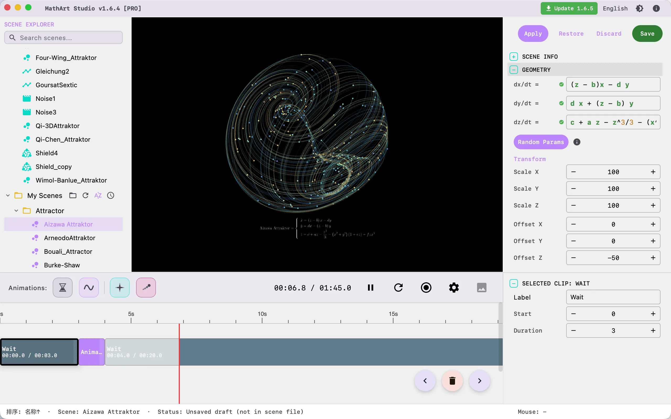
Interface Overview

All controls are located in the property panel on the right side, divided into seven main sections:

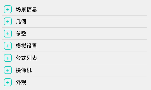
1. Geometry: Define differential equations, randomize parameters, and adjust spatial transforms
2. Parameters: Define custom constants used in equations
3. Simulation: Configure rendering mode, particle properties, and physics simulation parameters
4. Appearance: Adjust background color, point/line styles, and palette
5. Camera: Control viewing angle
6. Formulas: Display mathematical formulas and annotations
7. Scene Info: Edit scene name and description

---

Configuration Guide

1. Geometry (Differential Equations)

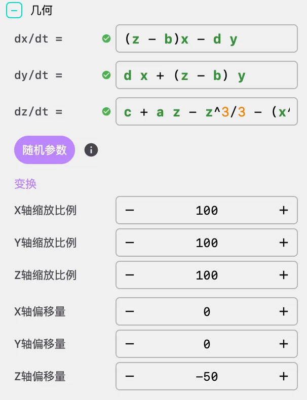
This is where you define the system's velocity field (Vector Field) — the core of the Strange Attractor scene.

Differential Equations

• dx / dy / dz: Define the differential equations for velocity components at position
  • Supported variables: x, y, z (spatial coordinates), and custom parameter names defined in the Parameters panel
  • Supported functions: sin, cos, tan, asin, acos, atan, sinh, cosh, tanh, sqrt, abs, log, ln, log10, exp, floor, ceil, round, sign, pow, min, max, atan2, etc.
  • Example (Aizawa system):
    • dx: (z - b) * x - d * y
    • dy: d * x + (z - b) * y
    • dz: c + a * z - z^3/3 - (x^2 + y^2) * (1 + e * z) + f * z * x^3

Tip: The equation input fields support syntax highlighting and autocomplete. Function names and variable names are displayed in different colors to help you quickly identify the equation structure.

Random Stable Parameters

This is one of the most powerful tools for exploring the attractor's parameter space. Click the "Random Stable" button, and the system performs an intelligent parameter search in the background:

1. Parameter Sensitivity Analysis: First analyzes the influence of each parameter on the system dynamics (calculating sensitivity through numerical differentiation)
2. Strategic Sampling: Performs targeted random perturbations around current parameter values, rather than blind random search
3. Stability Verification: For each candidate parameter set, executes short numerical integration (600 warmup steps + 3000 sampling steps) and evaluates:
   • Divergence ratio (≤ 2%)
   • Valid sample ratio (≥ 25%)
   • Coverage ratio (0.2% - 45%)
   • Whether collapsed to a line
   • Whether center offset is too large
4. Maximum 120 attempts, returning the highest-scoring stable parameter combination

Note: Random Stable only modifies equation parameters and will not change your adjusted spatial transforms (Scale/Offset). The search process runs in a background thread and does not block the UI.

Spatial Transforms

• Scale X/Y/Z: Adjust the size of the attractor in the scene
• Offset X/Y/Z: Adjust the position of the attractor in the scene
• Tip: Different attractor equations produce vastly different numerical ranges. Use Scale to adjust them to a suitable camera field of view. For example, the Aizawa attractor has a numerical range of approximately [-1.5, 1.5], requiring a larger Scale value (such as 60) to be clearly visible in the scene

---

2. Parameters (Custom Parameters)

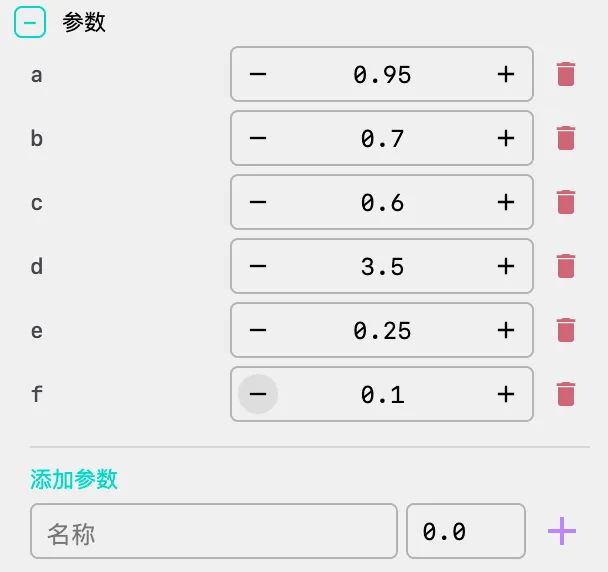
It is recommended to define named parameters here rather than hardcoding numbers in equations.

• Add Parameter: Enter a parameter name and default value, click the "+" button to create variables like sigma, rho, beta
• Usage: Use these variable names directly in the equations in the Geometry panel
• Real-time Adjustment: Modify these values during playback to dynamically evolve the attractor's shape
• Delete Parameter: Click the delete button to the right of a parameter to remove it
• Advantages:
  • Convenient for adjustment and experimentation
  • Supports parameter animation (via timeline)
  • Improves configuration readability and maintainability

Example: In the Aizawa attractor, define parameters a=0.95, b=0.7, c=0.6, d=3.5, e=0.25, f=0.1, then use these names in the equations — this is clearer and easier to adjust than writing numbers directly.

---

3. Simulation (Simulation Settings)

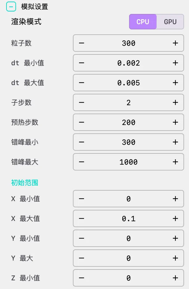
Control how the system evolves over time.

Rendering Mode

• CPU Mode:

  • Use case: Line and trail rendering
  • Features: Supports smooth, anti-aliased, variable-width trail drawing
  • Advantages: Suitable for high-quality video export
  • Limitation: Recommended particle count < 10,000 (for 60fps performance)
  • Trail support: Supports trail rendering

• GPU Mode:

  • Use case: Massive particle cloud rendering
  • Features: Uses GPGPU technology to simulate millions of particles
  • Advantages: Suitable for real-time performance and fluid-like density effects
  • Limitation: Does not support trail rendering
  • Trail support: No trails displayed in this mode

Particle Settings

• Particle Count: Number of independent particles in the system
  • Recommendations:
  • CPU mode: 500 - 5,000 (balance quality and performance)
  • GPU mode: 100,000 - 2,000,000 (fully utilize GPU performance)

Time Step

• dt_min / dt_max: Minimum/maximum integration step size
  • Purpose: Controls simulation precision and speed
  • Recommendations:
  • Smaller values (e.g., 0.005): More accurate simulation, but slower
  • Larger values (e.g., 0.02): Faster simulation, but potentially unstable
  • Randomization: Each particle is randomly assigned a time step within the [dt_min, dt_max] range, increasing visual diversity

Sub Steps

• Sub Steps: Number of physics calculations per rendered frame
  • Purpose: Controls simulation speed
  • Recommendations:
  • Increasing this value speeds up visual evolution while maintaining numerical stability
  • Typical values: CPU mode 2-10, GPU mode 2-5

Warmup Settings

• Warmup Steps: Number of pre-simulation steps before rendering the first frame

  • Purpose: Guides particles from initial random positions onto the attractor's orbit
  • Recommendation: At least 100 steps to avoid visual abruptness from random box distribution at the start

• Stagger Min/Max: Random additional warmup steps per particle

  • Purpose: Prevents all particles from clustering together at the start, creating a more natural distribution
  • Recommendation: Set to 1-1000 for natural distribution effects

Initialization Bounds

• Bounds: Defines the X/Y/Z coordinate range for initial particle generation
  • Default: Typically a small cube (e.g., [-0.1, 0.1]³)
  • Tip: The choice of initial positions affects warmup time and final distribution. Smaller initial ranges require more warmup steps but produce more uniform distributions

---

4. Appearance (Appearance Settings)

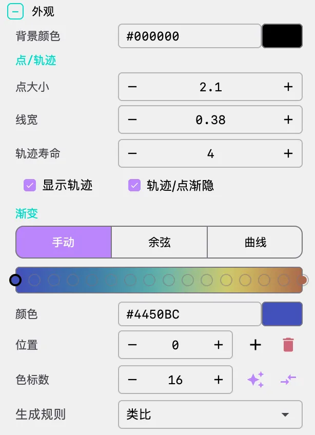
Adjust visual style.

Background Color

• Background Color: Set the rendering background color
  • Strange attractors typically use black or dark backgrounds to highlight particle and trail details

Points and Lines

• Dot Size: Diameter of particle heads
  • Recommendation: 1.0 - 3.0, adjusted based on particle count and visual effect
• Line Weight: Thickness of trail lines
  • Recommendation: 0.3 - 2.0, adjusted based on visual style

Trail Settings (CPU Mode Only)

• Trail Lifetime: Duration of trail history retention (seconds)
  • Recommendation: 3-10 seconds, balancing visual effect and memory usage
  • Warning: Excessively long lifetimes (>15 seconds) with many particles consume enormous memory
• Show Trails: Enable/disable trail rendering
• Fade Trails: When enabled, trails gradually become transparent over time
  • Effect: Produces softer, more natural visual results

Gradient Palette

Strange attractors support 1D LUT (lookup table) texture for coloring, with three gradient modes:

• Manual Mode:

  • Manually add, delete, and adjust color nodes
  • Supports drag-and-drop reordering of colors
  • Choose randomization strategies (monochromatic, analogous, complementary, split-complementary)
  • Click the ✨ button to quickly generate color schemes based on color theory

• Cosine Mode:

  • Uses the IQ cosine palette formula:
  • Separately control R/G/B channel bias, amplitude, frequency, and phase
  • Supports one-click randomization and application

• Curve Mode:

  • Control R/G/B channels separately through editable Bézier curves
  • Provides the most flexible color control
  • Click on empty space in the curve to add control points, double-click control points to delete
  • Supports one-click randomization and application

Tip: Particles select colors from the palette based on their index value. Use the "Randomize" button to quickly generate color schemes based on color theory.

---

5. Camera (Camera Controls)

Adjust the viewing angle and camera parameters.

Camera Angles

• Phi (Elevation): Camera's vertical angle

  • Range: 0 to π (0 to 180 degrees)
  • Purpose: Controls viewing the attractor from above or below
  • Default: π/2 (90 degrees, horizontal view)

• Theta (Azimuth): Camera's horizontal angle

  • Range: 0 to 2π (0 to 360 degrees)
  • Purpose: Controls camera rotation around the attractor
  • Default: 0

• Gamma (Roll): Camera's rotation angle

  • Range: 0 to 2π (0 to 360 degrees)
  • Purpose: Controls the camera's own rotation
  • Default: 0

Tips

• Multi-angle Observation: Adjust Phi and Theta to observe the attractor's 3D structure from different angles
• Animation Effects: Combine with the timeline system to create camera rotation animations
• Expression Support: Supports mathematical expressions (e.g., PI/2, PI/4)

---

6. Formulas (Formula Display)

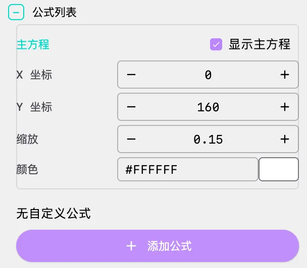
Display mathematical formulas and equations in the scene.

Main Equation Display

• Show Main Equation: Enable/disable main equation display

  • Purpose: Display the current attractor's differential equation system in the scene
  • Auto-generation: The system automatically generates LaTeX formulas based on current equations and parameters

• Main Equation Position:

  • X: Horizontal position coordinate
  • Y: Vertical position coordinate
  • Scale: Formula scaling ratio
  • Color: Formula color

Custom Formulas

You can add multiple custom formulas to the scene:

• Add Formula: Click the "Add Formula" button to add a new formula
• Formula Content:
  • LaTeX: Mathematical formula in LaTeX format
  • X: Horizontal position coordinate
  • Y: Vertical position coordinate
  • Scale: Formula scaling ratio
  • Color: Formula color
• Delete Formula: Click the delete button in the upper right corner of the formula to remove it

Use Cases

• Educational Display: Show the mathematical definition of the attractor in videos
• Annotations: Add notes or explanatory text
• Multi-formula Comparison: Display equations of multiple attractors simultaneously for comparison

LaTeX Syntax Tips

• Basic Syntax: Supports standard LaTeX mathematical formula syntax
• Examples:
  • \dot{x} = \sigma(y - x) displays dx/dt
  • \frac{dx}{dt} displays fraction form
  • \begin{cases} ... \end{cases} displays equation systems

---

7. Scene Info (Scene Information)

Edit the scene's metadata.

• Description: Add a text description for the scene, up to 300 characters
  • Character count is displayed in real-time below the input field
  • Description information is saved in the scene configuration file for easy management and retrieval

---

Animation and Timeline

Timeline System

The Strange Attractor scene fully supports the timeline system, enabling complex animation sequences.

Camera Animation

• Rotation: Rotate the camera around the attractor (rotateTheta)
• Align: Align the camera to a specific angle
• Zoom: Adjust camera distance (zoom)
• Focal Length: Adjust camera focal length (focal)
• Tracking: Track a specific particle (track)
• Ambient Light: Adjust scene ambient light (ambient)

Parameter Animation

• Parameter Changes: Dynamically modify equation parameters
• Effect: Attractor shape evolves over time
• Example: Dynamically change the rho parameter in the Lorenz system to observe the attractor's shape transformation

Configuration Method

Define animation sequences through the timeline array in the JSON configuration file:

{
  "timeline": [
    {
      "duration": 3,
      "label": "Wait",
      "type": "wait",
      "easing": "SINE_IN_OUT"
    },
    {
      "duration": 1,
      "label": "Animate",
      "type": "animate",
      "easing": "SINE_IN_OUT",
      "actions": [
        {
          "args": [0.2, 0.2, 0.2],
          "method": "ambient"
        }
      ]
    },
    {
      "duration": 20,
      "label": "Wait",
      "type": "wait",
      "easing": "SINE_IN_OUT"
    },
    {
      "duration": 7,
      "label": "Camera",
      "type": "animate",
      "easing": "SINE_IN_OUT",
      "actions": [
        { "args": [4], "method": "zoom" },
        { "args": [5], "method": "focal" }
      ]
    }
  ]
}

---

Performance and Best Practices

Recommended Configurations

Goal	Render Mode	Particles	Trail Lifetime	Sub Steps	Warmup Steps
High-quality video	CPU	1,000-2,000	5-10s	5-10	200+
Real-time interaction	GPU	100,000+	N/A	2-3	100+
Balanced performance	CPU	500-1,000	3-5s	4-6	100-200

Performance Optimization Tips

1. CPU Mode Optimization:

   • Reduce particle count (< 2,000)
   • Shorten trail lifetime (< 10 seconds)
   • Appropriately increase sub steps (5-10)

2. GPU Mode Optimization:

   • Increase particle count (100,000+)
   • Reduce sub steps (2-3)
   • Use smaller dot sizes

3. General Optimization:

   • Adjust time step to balance precision and speed
   • Set appropriate warmup steps to avoid visual abruptness
   • Use the "Random Stable" feature to quickly find parameter combinations with good visual quality

---

Common Issues

Particle Divergence/Explosion

Problem: Particles fly off to infinity, system crashes

Cause: Integration step dt is too large relative to the energy of the current equations

Solutions:

• Reduce dt_max (e.g., from 0.01 to 0.005)
• Check if equations are correct
• Ensure parameter values are within reasonable ranges
• Use the "Random Stable" button to search for stable parameter combinations

Discontinuous Trails

Problem: Trails appear broken or discontinuous

Cause: Too few sub steps or simulation speed too fast

Solutions:

• Increase sub_steps (e.g., from 2 to 8)
• Reduce time step
• Lower overall simulation speed

Out of Memory

Problem: Program crashes or runs slowly

Cause: Trail lifetime too long or too many particles

Solutions:

• Reduce trail_lifetime (e.g., from 20 seconds to 5 seconds)
• Reduce particle count
• Switch to GPU mode (GPU mode does not store trail history)

Poor Visual Quality

Problem: Attractor looks blurry or messy

Cause: Too many particles or dot size too large

Solutions:

• Reduce particle count
• Reduce dot size
• Adjust color scheme to increase contrast
• Enable Fade Trails for softer effects

Cannot Find Good Parameters

Problem: Manual parameter adjustment rarely produces aesthetically pleasing attractors

Solutions:

• Use the "Random Stable" button — the system automatically searches for parameter combinations that produce stable and visually meaningful attractors
• Start from classic attractor parameters and make small adjustments
• Ensure parameter values are within reasonable ranges (avoid extreme values)

---

Classic Attractor Examples

Aizawa Attractor

The Aizawa attractor is known for its unique rotational symmetry structure, resembling a disc with spiral arms.

{
  "equations": {
    "dx": "(z - b) * x - d * y",
    "dy": "d * x + (z - b) * y",
    "dz": "c + a * z - z^3/3 - (x^2 + y^2) * (1 + e * z) + f * z * x^3"
  },
  "parameters": {
    "a": 0.95,
    "b": 0.7,
    "c": 0.6,
    "d": 3.5,
    "e": 0.25,
    "f": 0.1
  }
}

Lorenz Attractor

The most classic strange attractor, discovered by meteorologist Edward Lorenz in 1963.

{
  "equations": {
    "dx": "sigma * (y - x)",
    "dy": "x * (rho - z) - y",
    "dz": "x * y - beta * z"
  },
  "parameters": {
    "sigma": 10.0,
    "rho": 28.0,
    "beta": 2.667
  }
}

Rössler Attractor

Proposed by Otto Rössler in 1976, it is a simplified version of the Lorenz system.

{
  "equations": {
    "dx": "-y - z",
    "dy": "x + a * y",
    "dz": "b + z * (x - c)"
  },
  "parameters": {
    "a": 0.2,
    "b": 0.2,
    "c": 5.7
  }
}

---

Gallery

---

Technical Details

Numerical Integration

The system uses Euler Integration for numerical computation:

x(t+dt) = x(t) + dx/dt * dt
y(t+dt) = y(t) + dy/dt * dt
z(t+dt) = z(t) + dz/dt * dt

This is the simplest yet effective integration method, suitable for real-time rendering. CPU mode uses Euler's method, while GPU mode uses the fourth-order Runge-Kutta method (RK4) for higher precision.

GPU Acceleration

GPU mode uses GLSL shaders for physics computation:

• Uses Ping-Pong texture technique for double buffering
• Updates all particle positions each frame
• Renders particles through vertex shaders

Thread Safety

CPU mode warmup and update processes use parallel computation:

• Utilizes multi-core CPU for accelerated computation
• ThreadLocal storage ensures thread safety
• Suitable for large-scale particle systems

Parameter Randomization Algorithm

AttractorParameterRandomizer employs a "sensitivity-guided local search + multi-metric numerical acceptance" strategy:

1. Parameter Sensitivity Analysis: Evaluates the influence of each parameter on system dynamics through numerical differentiation, including:

   • Total sensitivity (overall impact on dx, dy, dz)
   • XY plane sensitivity (impact on projection)
   • Z component sensitivity
   • Nonlinearity (variance of sensitivity across states)

2. Strategic Sampling: Performs targeted random perturbations around current parameter values, rather than blind search. Perturbation magnitude is dynamically adjusted based on sensitivity — parameters with high sensitivity receive smaller perturbations, while parameters with low sensitivity can explore a wider range

3. Multi-dimensional Acceptance: Verifies through short numerical integration whether candidate parameters produce stable, structured, and visually meaningful attractors. Evaluation metrics include divergence rate, escape rate, coverage, linearity, and center offset

4. Viewport Fit Suggestions: After the search completes, the system also calculates scale multiplier and offset increment suggestions to help fit the attractor graphic within an appropriate viewport range

---

Creative Tips

Parameter Exploration

1. Start with Classics: Use known classic parameter values first (e.g., Lorenz system σ=10, ρ=28, β=2.667)
2. Use Random Stable: Click the "Random Stable" button to let the system automatically search for interesting parameter combinations
3. Small Adjustments: Make small adjustments around classic values or random results
4. Observe Changes: Note the trends in attractor shape changes
5. Record Discoveries: Save interesting parameter combinations

Visual Design

1. Color Selection:

   • Use Cosine palette mode to quickly generate harmonious color schemes
   • Complementary colors highlight structure
   • Monochromatic tones create atmosphere
   • Dark backgrounds with high-saturation colors typically work best

2. Particle Count:

   • Few particles: Highlight individual trajectories, reveal motion details
   • Many particles: Reveal overall structure, present density distribution

3. Trail Effects:

   • Long trails: Reveal historical trajectories, present complete paths
   • Short trails: Focus on current positions
   • Fading trails: Soft transitions, more artistic

Animation Design

1. Camera Movement:

   • Slow rotation: Observe the attractor's 3D structure from all angles
   • Quick cuts: Dynamic effects
   • Aligned close-ups: Focus on details

2. Parameter Animation:

   • Slow changes: Observe evolution, understand parameter influence on shape
   • Fast changes: Produce sudden transformation effects
   • Cyclic changes: Create periodic animations

---

Mathematical Formula Reference

Common Functions

Function	Description	Example
sin, cos, tan	Trigonometric functions	sin(x), cos(y)
asin, acos, atan	Inverse trigonometric functions	atan(z)
sinh, cosh, tanh	Hyperbolic functions	tanh(x)
sqrt, abs	Square root, absolute value	sqrt(x*x + y*y)
log, ln, exp	Logarithm, exponential	exp(-x)
pow, min, max	Power, minimum, maximum	pow(x, 2)
floor, ceil, round	Rounding functions	floor(x)
sign	Sign function	sign(x)
atan2	Two-argument arctangent	atan2(y, x)

Operators

Operator	Description	Example
+, -, *, /	Arithmetic operations	x + y
%	Modulo	x % 2
^	Exponentiation	x ^ 2
(, )	Parentheses	(x + y) * z

---

Important Notes

1. Numerical Stability:

   • Excessively large time steps will cause the system to diverge
   • Start with smaller time steps
   • Observe particle motion and adjust parameters promptly

2. Memory Management:

   • Excessively long trail lifetimes consume enormous memory
   • GPU mode does not store trail history, suitable for many particles
   • Adjust particle count and trail lifetime based on available memory

3. Performance Balance:

   • CPU mode is suitable for high-quality rendering with fewer particles
   • GPU mode is suitable for real-time rendering with many particles
   • Choose the appropriate rendering mode based on your goals

4. Parameter Ranges:

   • Certain parameter combinations may cause system instability
   • Refer to classic attractor parameter ranges
   • Avoid extreme parameter values
   • Use the "Random Stable" feature to avoid unstable combinations

---

Advanced Topics

Custom Attractors

Steps to create a custom attractor:

1. Study the mathematical properties of the dynamical system
2. Design the differential equation system
3. Choose appropriate parameter ranges
4. Use the "Random Stable" feature to test numerical stability
5. Optimize visual effects

Chaos Theory Applications

Strange attractors are visualization tools for chaos theory:

• Demonstrate the unpredictability of deterministic systems
• Reveal complex behavior generated by simple rules
• Explore the boundary between order and disorder

Artistic Creation

Using strange attractors for artistic creation:

• Explore different parameter combinations
• Combine camera animation with parameter animation
• Experiment with different color schemes
• Create unique visual narratives

---

References

Mathematical Theory

• Strogatz, S. H. - Nonlinear Dynamics and Chaos
• Gleick, J. - Chaos: Making a New Science
• Lorenz, E. N. - Deterministic Nonperiodic Flow (1963)

Online Resources

• Wikipedia: Attractor
• Wikipedia: Lorenz system
• Wikipedia: Chaos theory

Software Documentation

• Processing 4 Official Documentation
• OpenGL Shader Programming Guide