Parametric Surface

Introduction

Parametric Surface Example

Parametric Surface is one of the most fundamental and powerful scene types in mathematical visualization. It maps a pair of parameters to 3D spatial coordinates , generating an infinite variety of curved geometries — from simple spheres and tori to complex helicoids, Möbius strips, and even stunning mathematical sculptures like the Cornucopia, all precisely expressible through parametric equations.

This scene supports two rendering modes: Particle Point Cloud (POINTS) and Mesh Surface (MESH), each suited to different creative needs. The particle mode excels at showcasing flow effects and trail animations, bringing surfaces to life; the mesh mode presents smooth surface geometry with support for fill, wireframe, materials, and procedural textures, ideal for displaying surface form and lighting effects.

Note: The Parametric Surface scene shares some UI components (such as camera controls, formula display, and gradient palettes) with Fractal, Map Attractor, and Symmetry Chaos scenes, but has its own independent equation input system, parameter domain controls, rendering pipeline, and animation controller, focused specifically on the creation and exploration of parametric surfaces.

Key Capabilities:

Free Equation Input: Write mathematical expressions directly in the x(u,v), y(u,v), z(u,v) input fields with real-time surface preview
Dual Rendering Modes: POINTS mode supports particle flow and trail effects; MESH mode supports fill, wireframe, materials, and procedural textures
CPU/GPU Dual Engine: CPU mode for high-precision rendering with trail effects; GPU mode for high-performance rendering with millions of particles
Custom Parameter System: Define parameters (e.g., a, R, r) in the Parameters panel and reference them directly in equations, supporting real-time adjustment and animation
Parameter Domain & Flow Control: Precisely control u, v parameter ranges with periodic boundaries and flow modes for perfect loop animations
Professional Palette: Supports manual, cosine, and curve gradient modes with automatic closed-loop detection for seamless coloring on closed surfaces
Full Animation Support: Parameter oscillation animation, camera animation, gradient animation, mode transition animation — all orchestrated through the timeline system

Mathematical Background

What is a Parametric Surface?

A parametric surface is a fundamental concept in differential geometry. Unlike implicit equations (e.g., defining a sphere), parametric surfaces map a 2D parameter domain to 3D space through three bivariate functions. This representation offers several advantages:

Intuitiveness: Each parameter value corresponds to a unique point on the surface, making the mapping between parameter domain and surface clear
Computability: Coordinates can be directly calculated from parameter values without solving equations
Samplability: Uniformly sampling the parameter domain easily generates mesh or point cloud representations of the surface
Animatability: Varying parameters over time creates the effect of particles flowing along the surface

Mathematical Definition of Parametric Surfaces

A parametric surface is defined by three bivariate functions:

where and form the parameter domain. You can think of the parameter domain as a piece of "fabric," and the parametric equations define how to "fold" this fabric into a surface in 3D space.

Classic Parametric Surfaces

Sphere:

The sphere is the most basic closed surface. Parameter u controls longitude (rotation around the Z-axis), and parameter v controls latitude (from north pole to south pole):

where , , and is the sphere radius.

Torus:

A torus is formed by combining a large circle (major circle) with a small circle (tube cross-section). Parameter u controls position along the major circle, and parameter v controls position along the tube cross-section:

where , , is the major radius, and is the minor radius.

Helicoid:

The helicoid is a classic example of a minimal surface — imagine a straight line rotating around an axis while simultaneously moving along the axis at a constant speed:

Möbius Strip:

The Möbius strip is the most famous non-orientable surface — it has only one side and one edge. It can be formed by twisting a strip of paper 180° and joining the ends:

where and .

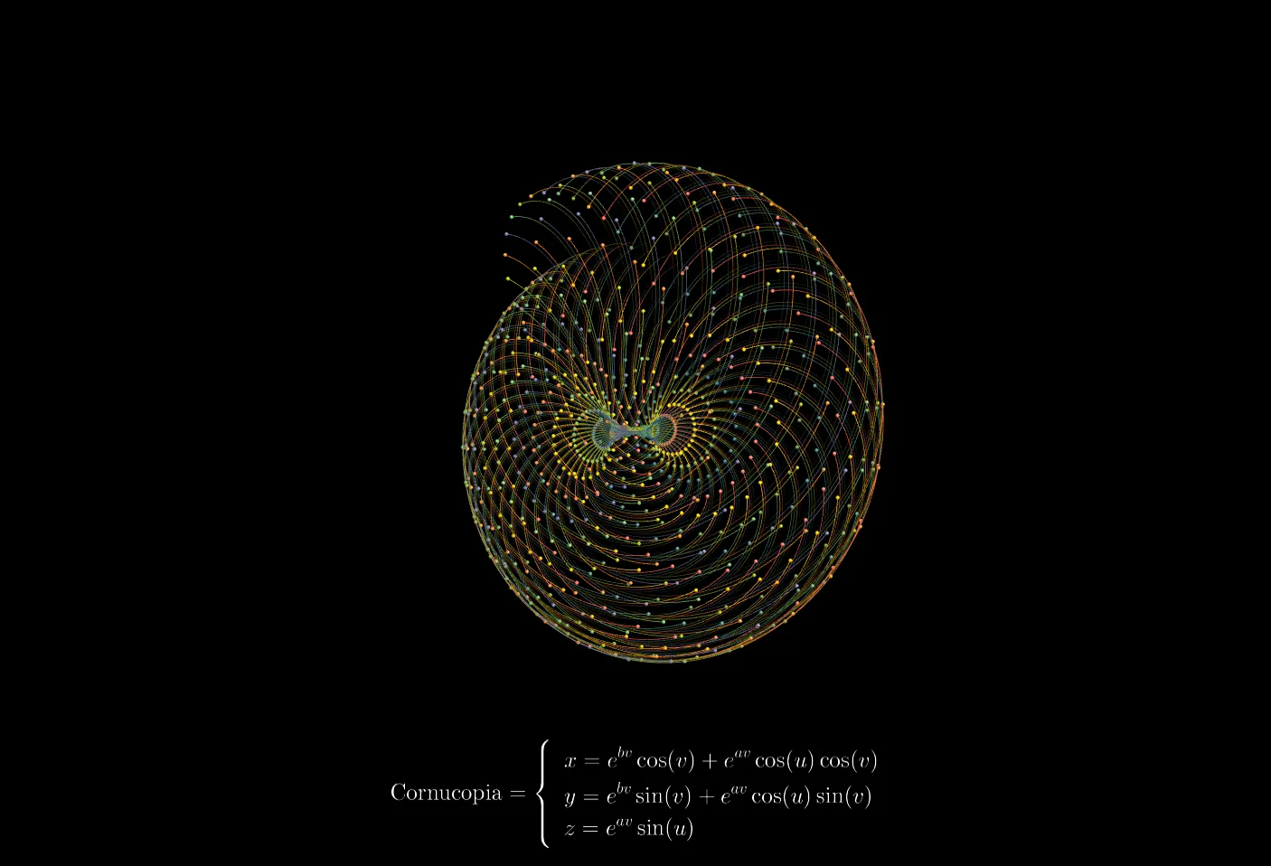
Cornucopia:

The Cornucopia is a spiral horn-shaped surface resembling the Horn of Plenty from Greek mythology. It uses exponential functions to achieve increasing radius, creating an elegant spiral unfolding effect:

where parameter controls the growth rate of the cross-section, and parameter controls the spiral expansion rate.

Relationship Between Parameter Domain and Surface Form

Parameter domain settings directly affect the surface form:

Parameter Domain	Suitable Surface	Description
,	Sphere	u traverses longitude once, v from north to south pole
,	Torus	Both parameters traverse a full circle
,	Helicoid	u controls radial range, v controls rotation
,	Möbius Strip	u must traverse two full circles to close

Historical Background

The study of parametric surfaces traces back to the early days of mathematics. In the 18th century, Leonhard Euler pioneered the systematic study of surface parameterization. In the 19th century, Carl Friedrich Gauss laid the foundations of differential geometry of surfaces in his Disquisitiones Generales circa Superficies Curvas (1827), introducing core concepts such as Gaussian curvature and proving the Theorema Egregium — that curvature is an intrinsic property of surfaces.

Bernhard Riemann further generalized Gauss's work, proposing the concepts of manifolds and Riemannian geometry, laying the groundwork for modern geometry. In the 20th century, parametric surfaces became a core tool in computer graphics — Bézier surfaces, NURBS surfaces, and others are special cases of parametric surfaces, widely used in CAD modeling, animation production, and scientific visualization.

Supported Mathematical Functions

The formula editor supports the following standard mathematical functions:

Category	Functions	Description
Trigonometric	`sin`, `cos`, `tan`, `asin`, `acos`, `atan`	Angles in radians
Hyperbolic	`sinh`, `cosh`, `tanh`	Hyperbolic sine, cosine, tangent
Exponential & Logarithmic	`exp`, `log`, `ln`, `log10`, `sqrt`	exp is natural exponential, log/ln is natural logarithm
Rounding	`floor`, `ceil`, `round`, `sign`	floor rounds down, ceil rounds up
Others	`abs`, `pow`, `min`, `max`, `atan2`	atan2(y,x) returns the argument of point (x,y)

Built-in Constants: PI (π ≈ 3.14159), TWO_PI (2π ≈ 6.28318)

Tip: Parameter domain input fields also support expressions such as 2*TWO_PI, PI/4, etc.

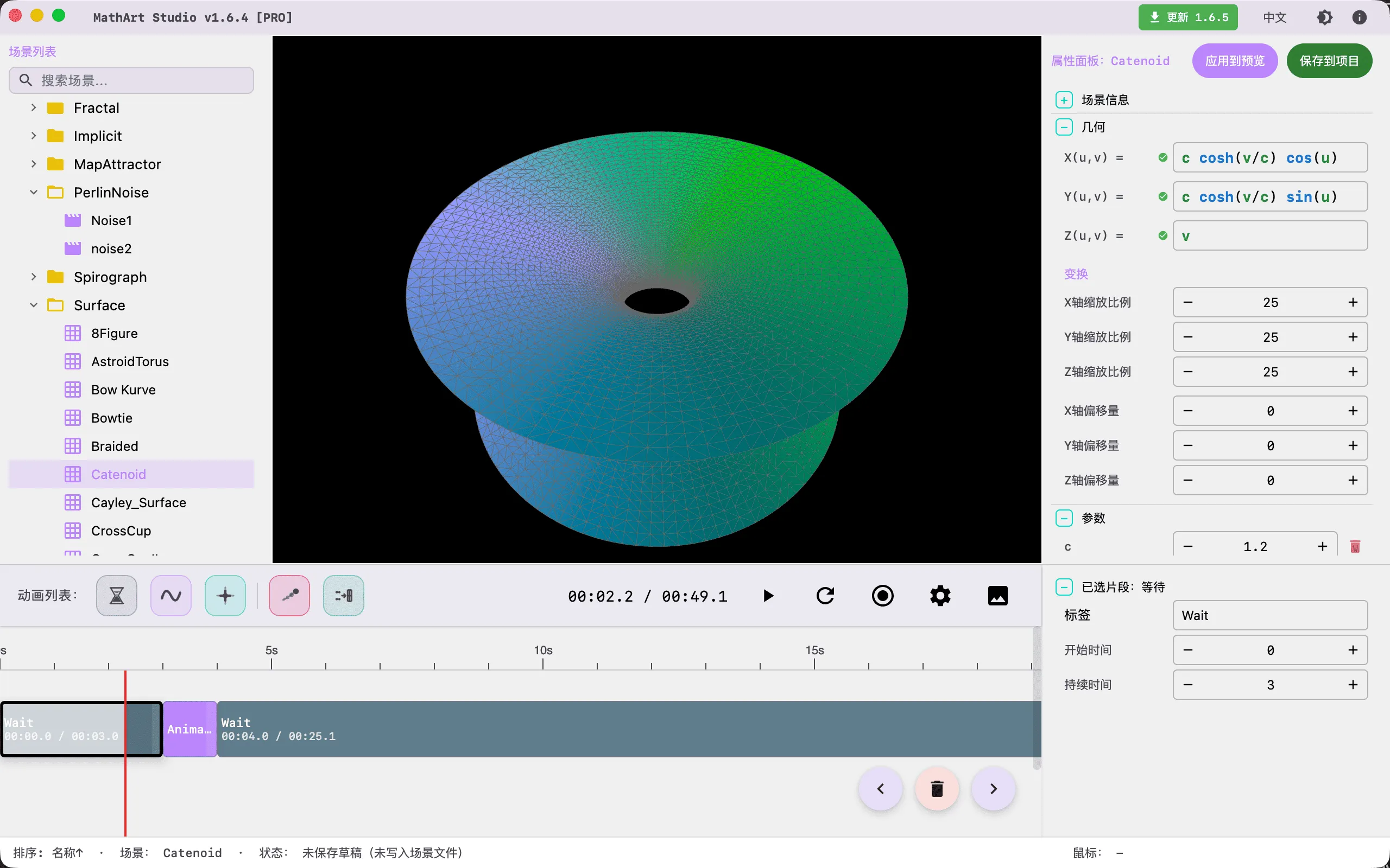
Interface Overview

All controls are located in the inspector panel on the right, divided into six main sections:

Geometry: Input surface equations, adjust spatial transforms
Settings: Select render mode, surface mode, configure parameter domain and simulation parameters
Camera: Control viewing angles
Formulas: Display mathematical formulas and annotations in the scene
Appearance: Adjust background color and gradient palettes
Parameters: Define custom constants used in equations

Configuration Guide

1. Geometry (Geometry Settings)

Geometry Settings

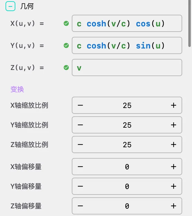
Equation Input

In the Geometry panel, define the parametric equations of the surface through three formula input fields:

x(u,v): Defines the coordinate function for the X-axis
y(u,v): Defines the coordinate function for the Y-axis
z(u,v): Defines the coordinate function for the Z-axis

Formulas can use variables u and v, as well as custom parameters (defined in the Parameters panel). For example, defining a torus:

x = (R + r * cos(v)) * cos(u)
y = (R + r * cos(v)) * sin(u)
z = r * sin(v)

where R and r are custom parameters defined in the Parameters panel.

Tip: Formula input fields support syntax highlighting and real-time validation. Invalid expressions will display a red border and error message.

Spatial Transform

Scale X/Y/Z: Scale multipliers in 3D space, default value 55.0
Offset X/Y/Z: Position offsets in 3D space, default value 0.0

Usage Tips:

Adjust scale to control the surface size in the scene
Adjust offset to position the surface anywhere in the scene
When the scene contains multiple geometries, use offset to precisely control their relative positions

2. Settings

Settings Panel

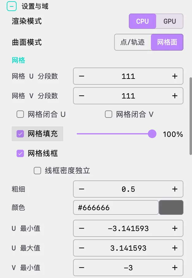
Render Mode

CPU: High-precision rendering, supports trails and line weight adjustment, ideal for high-quality video export
GPU: High-performance rendering, supports millions of particles, trails are disabled, ideal for real-time preview and massive point clouds

Important: GPU mode does not support trail effects. Switch to CPU mode if trails are needed.

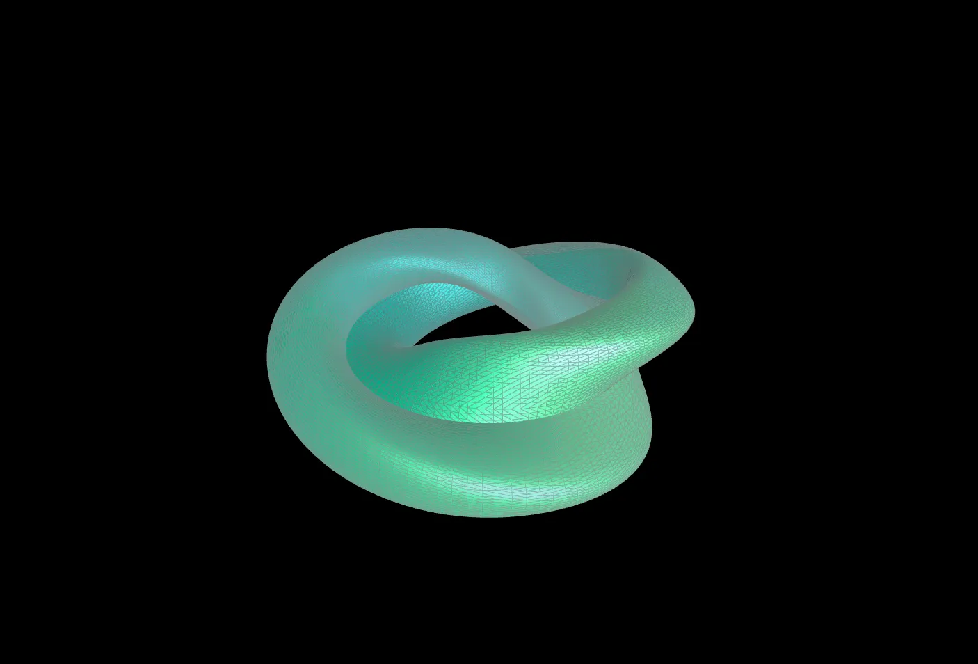
Surface Mode

POINTS: Particle point cloud mode, supports flow animation and trail effects
MESH: Mesh surface mode, supports fill, wireframe, materials, and procedural textures

MESH Mode Exclusive Parameters

Mesh Resolution:

Parameter	Description	Default	Minimum
u_segments	Number of mesh segments in U direction	60	2
v_segments	Number of mesh segments in V direction	60	2

Tip: Higher segment counts produce smoother surfaces but increase rendering overhead. Typically 60-100 segments are sufficiently smooth.

Wrapping Control (for closed surfaces):

Parameter	Description	Default
wrap_u	U-direction edge wrapping	Off
wrap_v	V-direction edge wrapping	Off
wrap_threshold	Wrapping detection threshold	0.25

Important: For closed surfaces (e.g., spheres, tori), you must enable wrap_u or wrap_v, otherwise the mesh will have gaps at the seams. wrap_threshold controls the sensitivity of seam detection — when the distance between endpoints is less than the threshold multiplied by the mesh diagonal length, the system automatically stitches them together.

Fill & Wireframe:

Parameter	Description	Default
fill	Enable mesh fill	On
fill_opacity	Fill opacity	90%
wireframe	Enable mesh wireframe	On
wireframe_decoupled	Decouple wireframe density	Off
wireframe_u_lines	U-direction wireframe lines (decoupled mode)	Same as u_segments
wireframe_v_lines	V-direction wireframe lines (decoupled mode)	Same as v_segments
wireframe_weight	Wireframe line weight	1.0
wireframe_color	Wireframe color	#FFFFFF

Tip: Enabling wireframe_decoupled allows independent control of wireframe density, unconstrained by mesh segment count. This is useful when you need fine mesh resolution but sparse wireframe lines.

Material & Texture (GPU MESH mode only):

Parameter	Description	Range
shininess	Material shininess, controls highlight sharpness	0-100
ambient	Ambient light color	Hex color value
specular	Specular highlight color	Hex color value
procedural_texture	Procedural texture type	See table below

Procedural Texture	Description
None	No texture, uses solid color fill
Checkerboard	Checkerboard pattern
Metal	Metal texture
Ceramic	Ceramic texture
Carbon	Carbon fiber texture

POINTS Mode Exclusive Parameters

Resolution:

Parameter	Description	Default
u_segments	Number of particles in U direction	60
v_segments	Number of particles in V direction	60

Important: Total particle count = u_segments × v_segments. Excessive resolution causes performance degradation. Recommended limits: CPU mode ≤ 100×100, GPU mode can reach 200×200 or higher.

Domain (Parameter Domain)

Parameter	Description	Example
u_min / u_max	Range of parameter u	Sphere: [0, 2π]
v_min / v_max	Range of parameter v	Sphere: [0, π]

Tip: Parameter domain input fields support mathematical expressions such as 2*TWO_PI, PI/4, -PI, etc.

Simulation (Simulation Parameters)

Parameter	Description	Default
speed_u	Motion speed of parameter u	0
speed_v	Motion speed of parameter v	0
periodic_u	U-direction periodic boundary	Off
periodic_v	V-direction periodic boundary	Off
flowing_u	U-direction flow mode	Off
flowing_v	V-direction flow mode	Off

Flow Mode Details:

flowing disabled (ping-pong mode): Particles bounce back and forth at parameter domain boundaries, producing a back-and-forth motion
flowing enabled (flow mode): Particles flow unidirectionally and loop seamlessly, ideal for perfect loop animations

Important: flowing mode must be used with periodic. If the surface is not closed (e.g., plane, helicoid), do not enable periodic, as this will produce incorrect visual results. Only enable periodic when the start and end of the parameter domain correspond to the same position on the surface (e.g., the u-direction of a sphere).

3. Camera (Camera Control)

Camera Settings

Adjust viewing angles and camera parameters. Unlike 2D scenes, parametric surfaces are true 3D objects, making camera control particularly important.

Camera Angles

Parameter	Description	Unit	Example
phi	Camera azimuth angle (horizontal rotation)	Radians	`PI/4`
theta	Camera polar angle (vertical rotation)	Radians	`PI/6`
gamma	Camera roll angle (rotation)	Radians	`0`

Tip: Camera angle input fields support mathematical expressions such as PI/4, PI/3. You can also use custom parameters for parameter-driven camera animation.

Common Viewing Angles:

View	phi	theta	Description
Front	0	0	View from directly in front
Top-down	PI/2	0	View from directly above
45° Isometric	PI/4	PI/4	Classic isometric view
Side	0	PI/2	View from the side

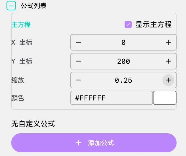
4. Formulas (Formula Display)

Formula Settings

Display LaTeX mathematical formulas in the scene for teaching demonstrations and documentation.

Main Equation

Parameter	Description	Default
show_main_equation	Whether to display the main equation	Off
x	X coordinate of the main equation display position	0
y	Y coordinate of the main equation display position	200
scale	Scale ratio of the main equation	1.0
color	Color of the main equation	#FFFFFF

Tip: The main equation is typically used to display the mathematical definition of the current surface. The system automatically generates LaTeX formulas based on the current equations.

Additional Formulas

Click the Add Formula button to add multiple formulas, each containing:

Parameter	Description	Example
latex	LaTeX format formula content	`x = r \cos(u) \sin(v)`
x	X coordinate of the formula display position	0
y	Y coordinate of the formula display position	300
scale	Scale ratio of the formula	1.0
color	Color of the formula	#FFFFFF

Applications:

Step-by-step demonstration of mathematical derivations
Display multiple related formulas
Add annotations and explanatory text

Note: Formula positions use screen coordinates with the top-left corner as origin, X-axis pointing right, and Y-axis pointing down.

5. Appearance (Appearance Settings)

Appearance Settings

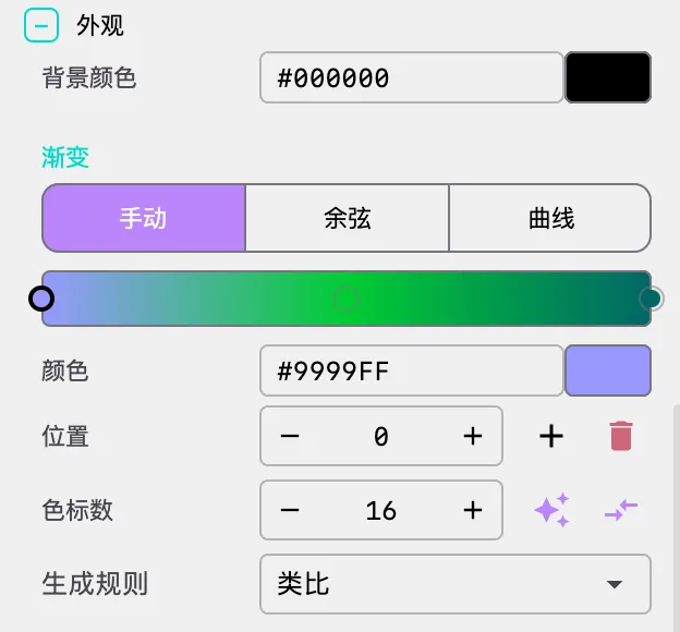
Background Color

background_color: Scene background color. Dark backgrounds (e.g., black #000000) typically highlight surface details and colors better.

Points & Lines (POINTS Mode)

Parameter	Description	Default
dot_size	Particle point size	1.68
line_weight	Trail line weight	1.0

Trail Effects (POINTS Mode, CPU Only)

Parameter	Description	Default	Recommended Range
show_trails	Show motion trails	Off	—
fade_trails	Trail fade-out effect	Off	—
trail_lifetime	Trail duration in seconds	5	5-10 seconds

Important Warning: trail_lifetime exceeding 15 seconds may cause excessive memory usage. Recommended range: 5-10 seconds.

Palette (Color Gradient)

Parametric surfaces use a 1D LUT (lookup table) texture for coloring, supporting three gradient modes:

Manual Mode:
- Click gradient bar to add color control points
- Drag control points to adjust positions
- Double-click control points to modify colors
- Supports up to 25 color control points
- Choose from random strategies (monochromatic, analogous, complementary, split-complementary)
Cosine Mode:
- Uses the IQ cosine palette formula: color(t) = a + b · cos(2π(c·t + d))
- Independently control offset, amplitude, frequency, and phase for R/G/B channels
- Supports one-click randomization and application
- Ideal for creating rainbow, metallic, and other continuous gradient effects
Curve Mode:
- Control R/G/B channels independently through editable Bézier curves
- Provides the most flexible color control
- Supports one-click randomization and application

Important: For closed surfaces, the system automatically detects and applies cyclic gradients to ensure smooth color transitions at seams. If issues persist, manually adjust the palette to ensure first and last colors match.

6. Parameters (Custom Parameters)

Parameters Settings

Define custom variables here that can be directly referenced in geometry formulas. Each parameter includes:

Name: Parameter name (e.g., a, R, r, etc.)
Value: Parameter value (supports decimals)

Adding Parameters: Enter the parameter name and initial value in the input fields at the bottom, then click the add button.

Deleting Parameters: Click the delete button to the right of the parameter.

Dynamic Effects: Modifying parameter values updates the surface shape in real-time, useful for:

Exploring the influence of parameters on surface morphology
Creating dynamic effects with parameter animation
Quickly switching between different parameter combinations

Animation and Timeline

Parametric surfaces support a rich set of animation types, and complex animation sequences can be orchestrated through the timeline system.

1. Parameter Flow Animation

By setting speed_u and speed_v, particles flow along parametric curves, creating fluid effects.

Configuration Steps:

Set speed_u and speed_v to non-zero values (e.g., 0.15) in the Settings panel
If the surface is closed, enable periodic_u and periodic_v
Enable flowing_u and flowing_v (for seamless looping)
Adjust trail_lifetime to control trail length (CPU mode)

Applications: Visualizing flow fields, magnetic field lines, contour flow on surfaces, etc.

2. Parameter Oscillation Animation

Through the paramStart / paramStop actions in the timeline, custom parameters undergo periodic sinusoidal oscillation within a specified range, achieving dynamic evolution of surface morphology.

How It Works:

For each parameter, specify the oscillation step and range (min, max)
The parameter value oscillates sinusoidally within [min, max]: value = mid + amp * sin(phase)
Oscillation speed is controlled by the step
Individual parameter oscillation can be enabled/disabled

Configuration Method:

Add a paramStart action in the timeline, then add the parameters to animate:

json

{
  "type": "animate",
  "duration": 10.0,
  "easing": "SINE_IN_OUT",
  "actions": [
    {
      "method": "paramStart",
      "args": [{
        "targetDomain": "SURFACE",
        "parameters": {
          "a": {
            "enable": true,
            "step": 0.01,
            "min": 0.02,
            "max": 0.08
          }
        }
      }]
    }
  ]
}

Animatable Parameters:

All custom parameters defined in the Parameters panel support animation. Additionally, the following domain parameters are supported:

Parameter	Description	Default Oscillation Range
scale	Overall scale	0.5 - 1.5
phaseDensity	Phase density	5.0 - 10.0
modDensity	Modulation density	5.0 - 10.0
phaseSharpness	Phase sharpness	0.001 - 2.0
modSharpness	Modulation sharpness	0.001 - 2.0

3. Camera Animation

Achieve view changes such as orbiting, zooming, and panning through the timeline system.

Available Camera Animation Methods:

Method	Description	Parameters
rotatePhi	Rotate azimuth angle	delta (radians increment)
rotateTheta	Rotate polar angle	delta (radians increment)
rotateGamma	Rotate roll angle	delta (radians increment)
rotateTo	Rotate to specified angles	phi, theta, gamma
zoom	Zoom	zoomLevel
focal	Adjust focal length	focalLength
track	Track particle	index
stopTracking	Stop tracking	None
ambient	Orbit rotation	phi_speed, theta_speed, gamma_speed
stopAmbient	Stop orbiting	None

4. Gradient Animation

Through gradientStart / gradientStop actions, palette colors change over time.

Gradient Animation Modes:

Mode	Description
HUE_ROTATE	Hue rotation, colors cycle along the color wheel
OFFSET_CYCLE	Offset cycle, colors shift along the gradient bar
CROSS_FADE	Cross fade
PALETTE_MORPH	Palette morphing

Interpolation Methods:

Method	Description
OKLAB	OKLAB color space interpolation (recommended, perceptually uniform)
OKLCH	OKLCH color space interpolation
LINEAR	Linear RGB interpolation
RGB	Standard RGB interpolation

5. Surface Mode Transition Animation

Through the SurfaceModeTransition animation type, you can smoothly transition between POINTS and MESH modes.

Configuration Method:

Add a SURFACE_MODE_TRANSITION type clip in the timeline and set the target mode (POINTS or MESH).

Configuration Example: Cornucopia Scene Animation

Here is a complete timeline configuration example demonstrating the animation choreography for the Cornucopia scene:

json

{
  "timeline": [
    {
      "type": "wait",
      "duration": 4.0,
      "easing": "SINE_IN_OUT"
    },
    {
      "type": "animate",
      "duration": 10.0,
      "easing": "SINE_IN_OUT",
      "actions": [
        {"method": "rotatePhi", "args": [6.283]}
      ]
    },
    {
      "type": "animate",
      "duration": 0.5,
      "easing": "SINE_IN_OUT",
      "actions": [
        {"method": "ambient", "args": [0.3, 0.3, 0.3]}
      ]
    },
    {
      "type": "animate",
      "duration": 5.0,
      "easing": "SINE_IN_OUT",
      "actions": [
        {"method": "zoom", "args": [5]},
        {"method": "focal", "args": [3.8]}
      ]
    },
    {
      "type": "animate",
      "duration": 5.0,
      "easing": "LINEAR",
      "actions": [
        {"method": "zoom", "args": [0.8]},
        {"method": "focal", "args": [25]}
      ]
    },
    {
      "type": "animate",
      "duration": 0.5,
      "easing": "SINE_IN_OUT",
      "actions": [
        {"method": "stopAmbient", "args": []}
      ]
    },
    {
      "type": "align",
      "duration": 12.0,
      "easing": "LINEAR",
      "target_phi": 0,
      "target_theta": 0,
      "target_gamma": 1.5708
    }
  ]
}

Classic Parametric Surface Examples

Cornucopia

The Cornucopia is the representative example of this scene, demonstrating how exponential functions create elegant spiral surfaces.

Equations:
x = exp(b*v) * cos(v) + exp(a*v) * cos(u) * cos(v)
y = exp(b*v) * sin(v) + exp(a*v) * cos(u) * sin(v)
z = exp(a*v) * sin(u)

Parameters: a = 0.05, b = 0.055
Domain: u ∈ [-2*TWO_PI, 2*TWO_PI], v ∈ [0, TWO_PI]
Render Mode: CPU, POINTS
Particles: 33 × 28
Flow Speed: speed_u = 0.15, speed_v = 0.15
Trails: enabled, fade, 5 seconds

Cornucopia Example

Sphere

Equations:
x = cos(u) * sin(v)
y = sin(u) * sin(v)
z = cos(v)

Domain: u ∈ [0, TWO_PI], v ∈ [0, PI]
Render Mode: GPU, MESH
Mesh Segments: 60 × 60
Wrapping: wrap_u = On, wrap_v = Off

Torus

Equations:
x = (R + r * cos(v)) * cos(u)
y = (R + r * cos(v)) * sin(u)
z = r * sin(v)

Parameters: R = 1.0, r = 0.4
Domain: u ∈ [0, TWO_PI], v ∈ [0, TWO_PI]
Render Mode: GPU, MESH
Wrapping: wrap_u = On, wrap_v = On

Möbius Strip

Equations:
x = (1 + t/2 * cos(u/2)) * cos(u)
y = (1 + t/2 * cos(u/2)) * sin(u)
z = t/2 * sin(u/2)

Domain: u ∈ [0, TWO_PI], t ∈ [-1, 1]
Render Mode: GPU, MESH
Note: The Möbius strip is non-orientable; wrap_u should not be enabled

Helicoid

Equations:
x = u * cos(v)
y = u * sin(v)
z = 0.5 * v

Domain: u ∈ [-2, 2], v ∈ [0, TWO_PI]
Render Mode: GPU, MESH
Flow Effect: speed_v = 0.2, periodic_v = On, flowing_v = On

Performance & Best Practices

Recommended Configurations

Goal	Render Mode	Surface Mode	Segments	Trails	Performance
High-quality video export	CPU	POINTS	50-100	5-10s	30-60 FPS
Real-time smooth preview	GPU	POINTS	200+	N/A	60+ FPS
Large-scale point clouds	GPU	POINTS	300+	N/A	30-60 FPS
Smooth surface display	GPU	MESH	60-100	—	60 FPS
Teaching demonstration	CPU	POINTS	30-50	5s	60 FPS

Performance Optimization Tips

Render Mode Selection:
- Need trail effects → Use CPU mode
- Need high-resolution particles → Use GPU mode
- Need materials and textures → Use GPU MESH mode
Resolution Control:
- Total particle count = u_segments × v_segments
- CPU mode recommended maximum: 100×100 (10,000 particles)
- GPU mode can reach 200×200 or higher (40,000+ particles)
- MESH mode: 60-100 segments are typically smooth enough
Trail Optimization:
- trail_lifetime should not be too long; recommended 5-10 seconds
- Enable fade_trails for natural trail fade-out with better visual results
- Excessively long trails consume significant memory
Closed Surface Handling:
- Correctly set parameter domain ranges (e.g., )
- Enable periodic_u or periodic_v (for POINTS mode flow)
- Enable wrap_u or wrap_v (for MESH mode stitching)
- Adjust wrap_threshold to optimize seams (default 0.25)

Troubleshooting

Interface Lag

Problem: Interface stutters or lags during operation

Cause: Too many particles or excessive trail duration

Solutions:

Reduce u_segments and v_segments
Reduce trail_lifetime
Switch to GPU mode (note: GPU mode does not support trails)

No Trail Effects

Problem: show_trails is enabled but no trails are visible

Cause: Running in GPU mode

Solution: Switch to CPU mode and enable show_trails

Mesh Gaps at Seams

Problem: In MESH mode, closed surfaces have gaps at the seams

Cause: Incorrect wrapping settings

Solutions:

Check if parameter domain ranges are correct (e.g., sphere )
Enable wrap_u or wrap_v
Adjust wrap_threshold value (increasing the threshold can stitch larger gaps)

Incomplete Surface Display

Problem: Only part of the surface is displayed

Cause: Improper parameter domain range settings

Solutions:

Check if u_min, u_max, v_min, v_max cover the complete parameter range
Check if Scale is too large causing the surface to extend beyond the viewport
Adjust Offset to bring the surface into view

Discontinuous Colors at Seams

Problem: Colors on closed surfaces show abrupt changes at seams

Cause: Palette not applying cyclic gradient

Solution: The system automatically detects closed surfaces and applies cyclic gradients. If issues persist, manually adjust the palette to ensure first and last colors match.

Formula Input Errors

Common Errors:

Misspelled function names (e.g., Sin should be sin, Cos should be cos)
Undefined parameter names (must define in Parameters panel before referencing in equations)
Mismatched parentheses
Division by zero or negative square roots

Solution: Check formula syntax, ensure all parameters are defined, and avoid mathematically illegal operations. Input fields display real-time validation results.

Abnormal Particle Flow Direction

Problem: Flow mode is enabled but particles move in unexpected directions

Cause: flowing mode not used with periodic, or periodic enabled on a non-closed surface

Solutions:

flowing mode must be used with periodic
Only enable periodic for closed surfaces (where parameter domain start and end correspond to the same position)
Non-closed surfaces should use ping-pong mode (do not enable flowing)

Creative Techniques

Parameter Exploration

Start from Classic Surfaces: Choose a classic surface (e.g., sphere, torus) as a starting point and gradually modify equations
Extract Parameters: Extract constants from equations as custom parameters for easy adjustment and animation
Small Steps: Modify only one parameter or one term in the equation at a time to observe changes
Mix Equations: Try combining equations from two surfaces to create new forms

Visual Tuning

Render Mode Selection:
- Display surface form → MESH mode with fill and wireframe
- Display flow effects → POINTS mode with CPU rendering and trails
- High particle density → POINTS mode with GPU rendering
Color Schemes:
- Use cosine palette mode to quickly generate harmonious color schemes
- Dark backgrounds with high-saturation colors typically produce the best results
- For closed surfaces, ensure first and last colors match
Camera Angles:
- 45° isometric view is suitable for displaying 3D form
- Camera orbit animation can showcase the surface from all angles
- Focal length adjustment can change perspective effects

Animation Design

Parameter Oscillation:
- Set oscillation animations for custom parameters to observe continuous morphological changes
- Different parameters oscillating at different rates create complex morphological evolution
- Ideal for creating morphing teaching animations
Particle Flow:
- Set speed_u and speed_v to make particles flow along the surface
- Combine with trail effects to show flow field direction
- Enable flowing mode for perfect loops
Camera Movement:
- Orbit animation (ambient) can showcase the surface from all angles
- Zoom animation can reveal fine structural details
- Tracking (track) can make the camera follow a specific particle
Gradient Animation:
- Hue rotation (HUE_ROTATE) creates rainbow flow effects
- Offset cycle (OFFSET_CYCLE) makes colors flow along the surface
- Combine with OKLAB interpolation for natural color transitions

Formula Writing Tips

Use Custom Parameters: Extract constants from formulas as parameters for easy adjustment and animation
Mind Parameter Ranges: Ensure formulas are well-defined throughout the parameter domain, avoiding division by zero, negative square roots, etc.
Utilize Periodicity: For periodic functions, parameter domains can be set to or
Piecewise Functions: Use min, max, abs functions to achieve piecewise effects
Exponential Functions: exp() can create increasing/decreasing spiral effects (e.g., Cornucopia)

Technical Details

Rendering Pipeline

Parametric surfaces use different rendering pipelines depending on render mode and surface mode:

POINTS + CPU Mode:

CPU calculates each particle's position
Supports trail effects: records particle history positions, draws as line segments
Supports line weight adjustment and fade effects
Ideal for high-quality video export

POINTS + GPU Mode:

GPU shaders compute particle positions in parallel
Uses textures to store particle state
Does not support trail effects
Supports real-time rendering of millions of particles

MESH Mode:

Generates triangle mesh based on segment count
Vertex shader computes mesh vertex positions
Fragment shader handles lighting, materials, and textures
Supports fill, wireframe, and procedural textures

Seam Stitching Algorithm

For closed surfaces, MESH mode uses a stitching algorithm to eliminate seams:

Detects mesh vertices at the start and end of the parameter domain
When the distance between endpoints is less than wrap_threshold × diagonal length, they are identified as the same vertex
Merges these vertices to generate a continuous triangle mesh
Automatically adjusts texture coordinates to ensure color continuity at seams

Parameter Animation System

Parameter animation for parametric surfaces is implemented through SurfaceParameterAnimator:

Supports sinusoidal oscillation animation for custom parameters
Each parameter independently controls step, range, and enable state
Animation parameters are passed to GPU shaders through Uniform variables without recompilation
Supports smooth start and stop

Advanced Topics

Understanding Geometric Properties of Parametric Surfaces

The geometric properties of parametric surfaces are determined by the first and second fundamental forms:

First Fundamental Form: Describes the metric on the surface (distances, angles, areas), determined by the inner products of partial derivatives and
Second Fundamental Form: Describes the curvature of the surface, determined by the surface normal and second-order partial derivatives
Gaussian Curvature: , where and are the principal curvatures. Points with positive Gaussian curvature are elliptic (e.g., sphere), negative are hyperbolic (e.g., saddle), and zero are parabolic (e.g., cylinder)

Creating Custom Surfaces

While the system provides equations for classic surfaces, you can create entirely new surface forms by modifying equations:

Deformation: Add perturbation terms to existing equations, e.g., x = ... + a * sin(3*u) * cos(2*v)
Blending: Weighted combination of two surface equations, e.g., x = t * f1(u,v) + (1-t) * f2(u,v)
Parameterization: Replace constants in equations with adjustable parameters to explore parameter space
Composition: Use the output of one surface as input to another

CPU vs GPU Mode Selection Strategy

Consideration	CPU Mode	GPU Mode
Trail effects	✅ Supported	❌ Not supported
Particle count	≤ 10,000	≤ 400,000+
Rendering precision	High	Medium
Real-time performance	Medium	High
Video export	Recommended	Available
Material textures	❌ Not supported	✅ Supported (MESH mode)

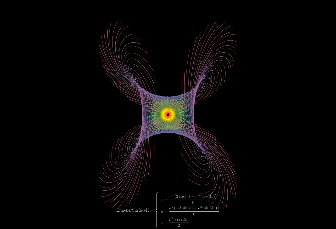
More Visual Examples

Parametric Surface Example 1 Parametric Surface Example 2

References

Mathematical Theory

Carl Friedrich Gauss - Disquisitiones Generales circa Superficies Curvas (1827)
Manfredo P. do Carmo - Differential Geometry of Curves and Surfaces
Erwin Kreyszig - Differential Geometry

Online Resources

Wikipedia: Parametric Surface
Wikipedia: Differential Geometry of Surfaces
MathWorld: Parametric Surface
3D Surface Gallery - Rich collection of parametric surface examples

Software Documentation

OpenGL Shader Programming Guide
GLSL Language Specification

Parametric Surface ​

Introduction ​

Mathematical Background ​

What is a Parametric Surface? ​

Mathematical Definition of Parametric Surfaces ​

Classic Parametric Surfaces ​

Relationship Between Parameter Domain and Surface Form ​

Historical Background ​

Supported Mathematical Functions ​

Interface Overview ​

Configuration Guide ​

1. Geometry (Geometry Settings) ​

Equation Input ​

Spatial Transform ​

2. Settings ​

Render Mode ​

Surface Mode ​

MESH Mode Exclusive Parameters ​

POINTS Mode Exclusive Parameters ​

Domain (Parameter Domain) ​

Simulation (Simulation Parameters) ​

3. Camera (Camera Control) ​

Camera Angles ​

4. Formulas (Formula Display) ​

Main Equation ​

Additional Formulas ​

5. Appearance (Appearance Settings) ​

Background Color ​

Points & Lines (POINTS Mode) ​

Trail Effects (POINTS Mode, CPU Only) ​

Palette (Color Gradient) ​

6. Parameters (Custom Parameters) ​

Animation and Timeline ​

1. Parameter Flow Animation ​

2. Parameter Oscillation Animation ​

3. Camera Animation ​

4. Gradient Animation ​

5. Surface Mode Transition Animation ​

Configuration Example: Cornucopia Scene Animation ​

Classic Parametric Surface Examples ​

Cornucopia ​

Sphere ​

Torus ​

Möbius Strip ​

Helicoid ​

Performance & Best Practices ​

Recommended Configurations ​

Performance Optimization Tips ​

Troubleshooting ​

Interface Lag ​

No Trail Effects ​

Mesh Gaps at Seams ​

Incomplete Surface Display ​

Discontinuous Colors at Seams ​

Formula Input Errors ​

Abnormal Particle Flow Direction ​

Creative Techniques ​

Parameter Exploration ​

Visual Tuning ​

Animation Design ​

Formula Writing Tips ​

Technical Details ​

Rendering Pipeline ​

Seam Stitching Algorithm ​

Parameter Animation System ​

Advanced Topics ​

Understanding Geometric Properties of Parametric Surfaces ​

Creating Custom Surfaces ​

CPU vs GPU Mode Selection Strategy ​

More Visual Examples ​

References ​

Mathematical Theory ​

Online Resources ​

Software Documentation ​

Parametric Surface

Introduction

Mathematical Background

What is a Parametric Surface?

Mathematical Definition of Parametric Surfaces

Classic Parametric Surfaces

Relationship Between Parameter Domain and Surface Form

Historical Background

Supported Mathematical Functions

Interface Overview

Configuration Guide

1. Geometry (Geometry Settings)

Equation Input

Spatial Transform

2. Settings

Render Mode

Surface Mode

MESH Mode Exclusive Parameters

POINTS Mode Exclusive Parameters

Domain (Parameter Domain)

Simulation (Simulation Parameters)

3. Camera (Camera Control)

Camera Angles

4. Formulas (Formula Display)

Main Equation

Additional Formulas

5. Appearance (Appearance Settings)

Background Color

Points & Lines (POINTS Mode)

Trail Effects (POINTS Mode, CPU Only)

Palette (Color Gradient)

6. Parameters (Custom Parameters)

Animation and Timeline

1. Parameter Flow Animation

2. Parameter Oscillation Animation

3. Camera Animation

4. Gradient Animation

5. Surface Mode Transition Animation

Configuration Example: Cornucopia Scene Animation

Classic Parametric Surface Examples

Cornucopia

Sphere

Torus

Möbius Strip

Helicoid

Performance & Best Practices

Recommended Configurations

Performance Optimization Tips

Troubleshooting

Interface Lag

No Trail Effects

Mesh Gaps at Seams

Incomplete Surface Display

Discontinuous Colors at Seams

Formula Input Errors

Abnormal Particle Flow Direction

Creative Techniques

Parameter Exploration

Visual Tuning

Animation Design

Formula Writing Tips

Technical Details

Rendering Pipeline

Seam Stitching Algorithm

Parameter Animation System

Advanced Topics

Understanding Geometric Properties of Parametric Surfaces

Creating Custom Surfaces

CPU vs GPU Mode Selection Strategy

More Visual Examples

References

Mathematical Theory

Online Resources

Software Documentation