Implicit Surface

Introduction

An implicit surface is a three-dimensional shape defined through a scalar field function. Unlike parametric surfaces that generate points through parameter mapping, implicit surfaces determine surface positions by solving the equation . This definition inherently gives implicit surfaces a "volume" concept — when multiple implicit objects approach each other, they naturally blend together, forming liquid-like or organic forms, which is the foundation of the famous "Metaball" effect.

From spheres and tori to the Gyroid triply periodic minimal surface, from Chmutov algebraic surfaces to the Klein bottle, implicit surfaces encompass a vast array of beautiful and profound three-dimensional forms found in mathematics. This scene allows you to explore and render these stunning mathematical surfaces in real-time by entering arbitrary implicit function expressions.

Key Capabilities:

• Free Equation Input: Directly enter any implicit function with a rich built-in math function library (trigonometric, exponential, logarithmic, rounding, etc.)
• Custom Parameter System: Define adjustable parameters in equations and control shape changes in real-time via sliders
• Dual Backend Rendering: CPU and GPU (OpenGL Compute Shader) Marching Cubes computation backends, balancing compatibility and performance
• Dual Render Modes: PREVIEW (point cloud) and WIREFRAME (mesh rendering), adapting to different workflow stages
• Professional Materials & Textures: GPU mode supports Phong lighting model and procedural textures (checkerboard, metal, ceramic, carbon fiber)
• Full Animation Support: Integrated parameter oscillation animation system for smooth periodic parameter changes
• Palette System: Supports manual, cosine, and curve gradient modes, combined with JSON palettes for rich color expression

---

Mathematical Background

What is an Implicit Surface?

The core concept of implicit surfaces is the isosurface. Given a three-dimensional scalar field function , an isosurface is the set of all points satisfying , where is a constant (typically ).

Intuitively, you can think of as a "density value" or "potential value" at each point in 3D space, and the isosurface is the set of all points where the density equals a specific threshold — just like contour lines on a topographic map, but in three dimensions.

Implicit Surfaces vs. Parametric Surfaces:

Feature	Implicit Surface	Parametric Surface
Definition
Point-on-surface test	Direct substitution	Requires solving for parameters
Blending effects	Naturally supported (function addition)	Requires additional processing
Topology changes	Handled naturally	Difficult
Typical applications	Metaballs, algebraic surfaces	NURBS modeling

Common Implicit Functions

Name	Formula	Description
Sphere		Sphere with radius r
Ellipsoid		Semi-axes a, b, c
Cylinder		Infinite along Z-axis
Cone		Vertex at origin
Torus		Major radius R, minor radius r
Gyroid		Triply periodic minimal surface
Chmutov Surface		Based on Chebyshev polynomials

Marching Cubes Algorithm

This scene uses the classic Marching Cubes algorithm to extract triangular meshes from implicit functions. The algorithm was published by William E. Lorensen and Harvey E. Cline at SIGGRAPH in 1987 and remains the standard method for isosurface extraction.

Algorithm Principles:

1. Space Partitioning: Divide the 3D sampling space into a uniform voxel grid
2. Function Evaluation: Compute the implicit function value at each of the 8 vertices of every voxel
3. Isosurface Crossing Detection: Based on whether each vertex's function value is above or below the isovalue (typically 0), determine how the isosurface crosses through each voxel
4. Triangle Generation: Use a precomputed lookup table (256 cases) to generate triangular faces within each voxel
5. Vertex Interpolation: Determine precise triangle vertex positions through linear interpolation

CPU vs. GPU Backend:

Feature	CPU Backend	GPU Backend
Computation	Serial per-voxel computation	OpenGL Compute Shader parallel computation
Compatibility	All platforms	Requires OpenGL 4.3+
Speed	Adequate at low resolution	Significantly faster at high resolution
Render Modes	PREVIEW + WIREFRAME	WIREFRAME only
Material/Texture	Not supported	Supports Phong lighting + procedural textures

Historical Background

The study of implicit surfaces traces back to 19th-century algebraic geometry. Mathematicians investigated algebraic surfaces defined by polynomial equations , exploring their topological properties and singularity structures.

After Lorensen and Cline invented the Marching Cubes algorithm in 1987, implicit surfaces found widespread application in computer graphics. The algorithm made it possible to extract 3D organ models from medical CT/MRI data, and also gave rise to "Metaball" technology — proposed by Jim Blinn in 1982, which simulates organic blending effects by adding multiple potential functions together.

In mathematics, Chmutov surfaces (named after Russian mathematician Sergei Chmutov) are a class of algebraic surfaces based on Chebyshev polynomials, possessing rich symmetry and singularity structures, making them classic objects in algebraic surface research.

---

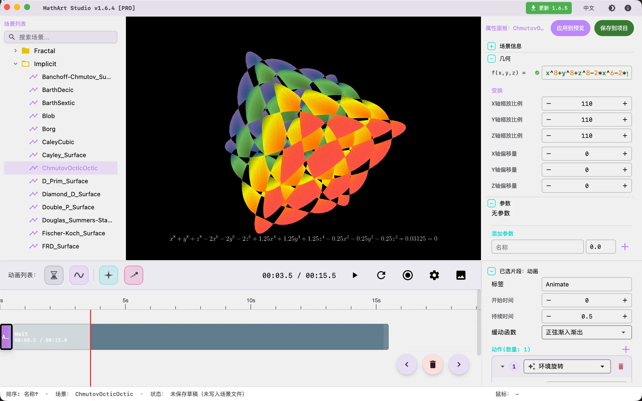
Interface Overview

All controls are located in the inspector panel on the right, divided into six main sections:

1. Geometry: Define the implicit function and spatial transformation parameters
2. Parameters: Define custom constants for dynamic shape control
3. Settings: Configure sampling domain bounds, resolution, render backend, and render mode
4. Camera: Control viewing angle
5. Formulas: Display mathematical formulas in the render
6. Appearance: Adjust background color and gradient palettes

---

Configuration Guide

1. Geometry (Geometry Settings)

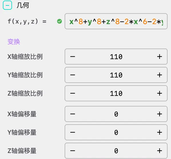
Implicit Equation Input

Enter the implicit function expression in the f(x, y, z) input field. The surface is generated where this function equals 0.

Supported Math Functions:

Category	Functions
Trigonometric	sin, cos, tan, asin, acos, atan, arcsin, arccos, arctan
Hyperbolic	sinh, cosh, tanh
Mathematical	sqrt, abs, log, ln, log10, exp
Rounding	floor, ceil, round, sign
Other	pow, min, max, atan2

Variables: Default available variables are x, y, z. Parameters defined in the Parameters panel also become available variables automatically.

Example Equations:

• Sphere: x*x + y*y + z*z - r*r
• Heart Surface: pow(x*x + 2.25*y*y + z*z - 1, 3) - x*x*z*z*z - 0.1125*y*y*z*z*z
• Klein Bottle: (x*x + y*y + z*z + 2*y - 1) * ((x*x + y*y + z*z - 2*y - 1)^2 - 8*z*z) + 16*x*z*(x*x + y*y + z*z - 2*y - 1)
• Chmutov Octic (this guide's example): x^8+y^8+z^8-2*x^6-2*y^6-2*z^6+1.25*x^4+1.25*y^4+1.25*z^4-0.25*x^2-0.25*y^2-0.25*z^2+0.03125

Tip: The equation input field supports syntax highlighting and real-time validation. After entering, press Enter or click the "Apply" button at the top of the panel to update the surface.

Spatial Transform

Parameter	Description	Default	Step
scale_x	X-axis scale multiplier	1.0	10
scale_y	Y-axis scale multiplier	1.0	10
scale_z	Z-axis scale multiplier	1.0	10
offset_x	X-axis position offset	0.0	10
offset_y	Y-axis position offset	0.0	10
offset_z	Z-axis position offset	0.0	10

Scaling and offset are applied after mesh generation to adjust the final render position and size. In the Chmutov Octic example, all three axes are scaled to 80, presenting the surface at an appropriate size in the viewport.

---

2. Parameters (Custom Parameters)

Custom variables defined in this section can be directly referenced in the f(x, y, z) formula. Modifying parameter values updates the surface shape in real-time.

Use Cases:

• Define adjustable radius: r = 1.5, then use x*x + y*y + z*z - r*r in the formula
• Create animation parameters: Drive parameter changes through timeline animations to achieve morphing effects
• Control complex shape features: Such as torus inner/outer radii, Gyroid periods, etc.

How to Use:

1. Enter a parameter name in the name input field (e.g., r, a, freq)
2. Set the initial parameter value in the value input field
3. Click the "+" button to add the parameter
4. Reference the parameter in your formula
5. Click the delete button on the right side of a parameter to remove it

Note: Parameter names must be valid variable names (starting with a letter, may contain digits) and cannot duplicate built-in variables x, y, z.

---

3. Settings (Domain & Resolution)

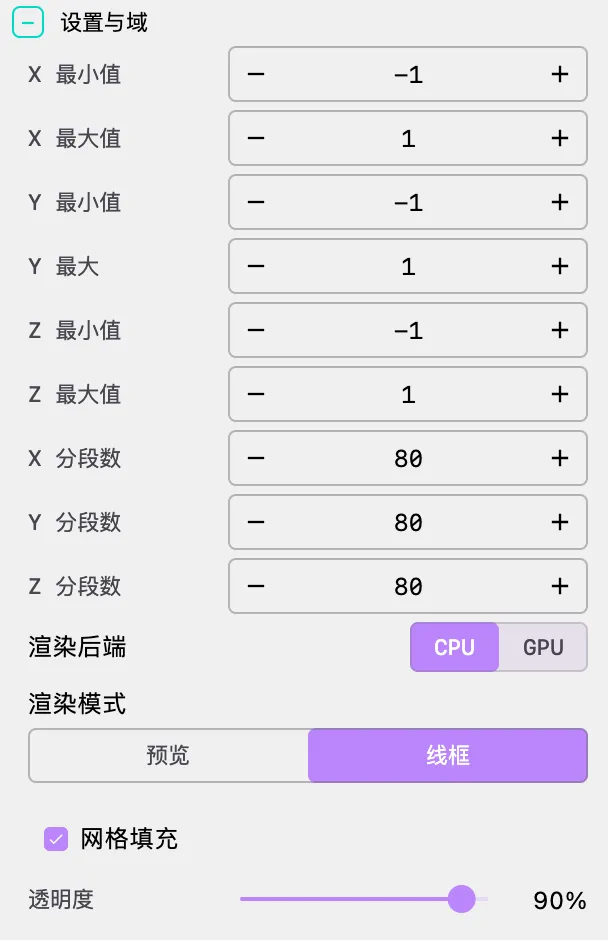
Bounds (Sampling Region)

Parameter	Description	Default	Precision
x_min / x_max	X-axis sampling range	-2 / 2	6 decimal places
y_min / y_max	Y-axis sampling range	-2 / 2	6 decimal places
z_min / z_max	Z-axis sampling range	-2 / 2	6 decimal places

Important: The sampling bounds define the 3D box region where the function is evaluated. Surface portions outside this range will be clipped. Ensure the bounds are large enough to cover the entire surface.

In the Chmutov Octic example, since the surface lies within the unit sphere, a sampling range of -1 to 1 fully covers it.

Resolution

Parameter	Description	Default
x_seg	X-axis voxel count	60
y_seg	Y-axis voxel count	60
z_seg	Z-axis voxel count	60

Performance Warning: The total voxel count is . Doubling all three dimensions increases computational load by 8×. Start with low values (40-60) for shape debugging, then increase resolution for final rendering.

Resolution	Voxel Count	Use Case
40 × 40 × 40	64,000	Quick preview
60 × 60 × 60	216,000	Regular editing
80 × 80 × 80	512,000	High-quality preview
100 × 100 × 100	1,000,000	High-quality rendering
150 × 150 × 150	3,375,000	Final output (requires patience)

The Chmutov Octic example uses 80 × 80 × 80 resolution, achieving a good balance between precision and performance.

Render Backend

Option	Description
CPU	Uses CPU for Marching Cubes computation. Good compatibility, supports both PREVIEW and WIREFRAME render modes
GPU	Uses OpenGL Compute Shaders for parallel computation. Fast, suitable for high-resolution rendering, but only supports WIREFRAME mode

Note: GPU mode requires OpenGL 4.3+ support. If you encounter issues, switch to CPU mode.

Render Mode

Mode	Description	Use Case
PREVIEW	Renders point cloud on the surface	Quick shape preview, parameter adjustment (CPU backend only)
WIREFRAME	Renders polygon mesh	Topology inspection, final output

Mesh Settings

When render mode is WIREFRAME, the following options are available:

Parameter	Description	Default
mesh_fill	Enable surface fill	On
opacity	Fill opacity (0% - 100%)	85%

Material Properties (GPU + WIREFRAME mode only):

Parameter	Description	Default
shininess	Material shininess (0 - 100), controls the size and intensity of specular highlights	32
ambient	Ambient light color	#4D4D4D
specular	Specular highlight color	#FFFFFF

Phong Lighting Model: GPU mode uses the classic Phong lighting model with three components: ambient, diffuse, and specular. shininess controls the focus of specular reflection — higher values produce more concentrated highlights, making the surface appear smoother.

Procedural Textures (GPU + WIREFRAME mode only):

Option	Description
None	No texture, uses solid color
Check	Checkerboard texture
Metal	Metallic texture
Ceramic	Ceramic texture
Carbon	Carbon fiber texture

---

4. Camera (Camera Control)

Adjust viewing angles and camera parameters. The camera uses spherical coordinates to define position and orientation relative to the scene origin.

Angle Parameters

Parameter	Description	Unit
phi	Pitch angle, the angle between the camera and the XY plane. Positive values point upward, negative values point downward	Radians
theta	Yaw angle, the camera's rotation angle on the XY plane	Radians
gamma	Roll angle, the camera's rotation around its own viewing axis	Radians

Common View Presets:

View	phi	theta	Description
Front View	0	0	View from positive Y-axis
Top View	π/2	0	View from positive Z-axis
Isometric View	π/4	π/4	Classic 45° isometric angle

Note: Camera parameters support mathematical expressions. You can use PI, sin(), cos(), and other functions. For example, PI/4 represents 45 degrees. The Chmutov Octic example uses phi = PI/2 (top view) to showcase the surface's symmetric structure.

---

5. Formulas (Formula Display)

Display mathematical formulas in the scene for annotation, educational demonstrations, or enhancing visual effects.

Main Equation Display

Parameter	Description	Default
show_main_equation	Whether to display the main equation	On
x	X coordinate of formula display position (pixels)	0
y	Y coordinate of formula display position (pixels)	0
scale	Formula scale ratio	1.0
color	Formula color (hexadecimal)	#FFFFFF

Position Note: The coordinate origin is at the top-left corner of the canvas. X-axis points right, Y-axis points down.

In the Chmutov Octic example, the main equation is displayed at the top of the viewport (y = 200), scaled to 0.25, in white text.

Custom Formulas

In addition to the main equation, you can add multiple custom formulas for displaying derivation processes, auxiliary explanations, or multiple related formulas. Click the "Add Formula" button to create a new formula item, each containing LaTeX content, position, scale, and color settings.

LaTeX Syntax Support:

• Basic operations: x^2, \frac{a}{b}, \sqrt{x}
• Greek letters: \alpha, \beta, \gamma, \theta, \phi
• Special symbols: \infty, \sum, \int, \partial
• Matrices: \begin{pmatrix} a & b \\ c & d \end{pmatrix}

---

6. Appearance (Appearance Settings)

Background Color

Sets the render background color. Implicit surfaces typically use black or dark backgrounds to highlight surface details and lighting effects.

Gradient Palette

Implicit surfaces use a 1D LUT (lookup table) texture for coloring. Surface colors are gradient-mapped based on Z-axis coordinates, from z_min to z_max corresponding to the palette's start to end. Three gradient modes are supported:

• Manual Mode:

  • Manually add, delete, and adjust color stops
  • Supports drag-and-drop reordering of colors
  • Choose from random strategies (monochromatic, analogous, complementary, split-complementary)

• Cosine Mode:

  • Uses the IQ cosine palette formula:
  • Independently control offset, amplitude, frequency, and phase for R/G/B channels
  • Supports one-click randomization and application

• Curve Mode:

  • Control R/G/B channels independently through editable Bézier curves
  • Provides the most flexible color control
  • Supports one-click randomization and application

The Chmutov Octic example uses a 7-color manual palette: from red to purple, presenting rich color layers.

---

Animation and Timeline

Implicit surfaces support parameter oscillation animation, allowing timeline-driven periodic parameter changes to achieve morphing effects.

Parameter Oscillation Animation

How It Works

Parameter oscillation animation is implemented through ImplicitSurfaceParameterAnimator:

1. For each parameter, specify the oscillation step, range (min, max), and edge easing
2. The parameter value oscillates sinusoidally within [min, max]:
3. Oscillation speed is jointly controlled by the step and step scale factor
4. Edge easing ensures the parameter decelerates near range boundaries, avoiding abrupt changes

Animation Configuration

In the JSON configuration file's timeline, use paramStart and paramStop actions to control parameter animation:

{
  "timeline": [
    {
      "type": "animate",
      "duration": 5.0,
      "actions": [
        {
          "method": "paramStart",
          "args": {
            "parameters": {
              "r": {
                "step": 0.05,
                "min": 0.5,
                "max": 2.0
              }
            }
          }
        }
      ]
    }
  ]
}

Parameter Animation Properties

Property	Description
step	Parameter change per frame. Positive for forward, negative for reverse
min	Parameter minimum value
max	Parameter maximum value
enable	Enable animation for this parameter (default: true)

Edge Easing

Parameter animation supports edge easing, allowing smooth deceleration as parameters approach boundary values, avoiding abrupt reversals:

{
  "edgeEasing": {
    "attackRatio": 0.3,
    "releaseRatio": 0.4,
    "easing": "SINE_OUT"
  }
}

Property	Description	Default
attackRatio	Easing zone ratio when approaching minimum	0.3
releaseRatio	Easing zone ratio when approaching maximum	0.4
easing	Easing function type	SINE_OUT

Camera Animation

Implicit surfaces also support standard camera animations:

• Rotation: Rotate camera around the surface
• Alignment: Align camera to specific angles
• Zoom: Adjust camera distance

Configuration Method

Define animation sequences through the timeline array in JSON configuration:

{
  "timeline": [
    {
      "type": "animate",
      "duration": 15.0,
      "easing": "SINE_IN_OUT",
      "actions": [
        {"method": "rotateTheta", "args": [6.283]}
      ]
    },
    {
      "type": "hold",
      "duration": 2.0
    }
  ]
}

The Chmutov Octic example includes an ambient light animation and a wait period, providing subtle lighting changes during display.

---

Performance & Best Practices

Recommended Configurations

Goal	Resolution	Backend	Render Mode	Estimated Time
Quick Preview	40-60	CPU	PREVIEW	< 1 second
Regular Editing	60-80	CPU or GPU	WIREFRAME	1-5 seconds
High-Quality Rendering	80-120	GPU	WIREFRAME	5-30 seconds
Final Output	120-150	GPU	WIREFRAME	30+ seconds

Performance Optimization Tips

1. Resolution Adjustment:

   • Reducing resolution is the most direct performance optimization
   • Total voxels = ; doubling all three dimensions increases computation by 8×
   • Start with low resolution to confirm the shape is correct, then gradually increase

2. Render Backend Selection:

   • CPU backend supports PREVIEW mode, suitable for quick previews
   • GPU backend is significantly faster at high resolutions, but requires OpenGL 4.3+ support
   • GPU mode only supports WIREFRAME rendering

3. Sampling Range Optimization:

   • Narrowing the sampling range reduces unnecessary computation
   • Ensure the range just covers the surface, avoiding overly large empty regions
   • For example, the sphere x*x + y*y + z*z - 1 only needs a range of -1.5 to 1.5

4. Memory Management:

   • High resolution consumes significant memory; recommend 16GB+ RAM for 150+ resolution
   • If the program crashes, try reducing resolution or using CPU mode

---

Creative Techniques

Shape Design

1. Start Simple:

   • Begin with a sphere x*x + y*y + z*z - r*r to verify settings are correct
   • Confirm sampling bounds and resolution are reasonable before trying complex shapes

2. Blending Effects:

   • Implicit surfaces naturally support blending — simply add potential functions together
   • Example (two spheres blending): (x*x + y*y + z*z - r1*r1) * ((x-d)*(x-d) + y*y + z*z - r2*r2) - c
   • Adjust parameter c to control blending degree

3. Sharp Edges:

   • Use min() or max() functions to create sharp edges
   • Example: min(x*x + y*y + z*z - 1, x*x + y*y - 0.25) creates the intersection of a sphere and cylinder

4. Leverage Parameter Animation:

   • Set oscillation animations for parameters to observe continuous morphological evolution
   • Suitable for creating animations that transition from one form to another

Visual Tuning

1. Lighting & Materials:

   • Use GPU + WIREFRAME mode for the best visual results
   • Adjust shininess to control highlight intensity — high values (80-100) for metallic surfaces, low values (10-30) for matte surfaces
   • Procedural textures can enhance realism: metal texture for hard surfaces, ceramic texture for smooth surfaces

2. Color Schemes:

   • Use cosine palette mode to quickly generate harmonious color schemes
   • Z-axis gradient mapping can highlight the surface's height layers
   • Dark backgrounds with high-saturation colors typically produce the best results

3. Camera Angles:

   • For symmetric surfaces (like Chmutov surfaces), top view (phi = π/2) best showcases symmetry
   • Isometric view (phi = π/4, theta = π/4) is suitable for showing 3D depth
   • Combine with camera rotation animation for a full 360° surface showcase

---

Troubleshooting

Empty Scene

Possible Causes:

1. Insufficient sampling bounds: Check if x_min/max, y_min/max, z_min/max cover the entire surface
2. No solution to equation: Confirm has a solution within the given range
   • Example: x*x + 1 is always positive, no solution
3. Resolution too low: If the surface is very thin, higher resolution may be needed to capture it

Solutions:

• First expand sampling bounds (e.g., -5 to 5) to confirm the surface exists
• Gradually narrow the bounds for better detail

Slow Performance

Possible Causes:

1. Resolution too high
2. Using CPU mode for high resolution

Solutions:

• Reduce x_seg, y_seg, z_seg
• Switch to GPU mode
• 200 × 200 × 200 resolution creates 8 million voxels with extremely heavy computation

Clipped Shape

Cause: Surface extends beyond sampling bounds

Solutions:

• Expand x_min/x_max and other boundary values
• Check if scale parameters cause the surface to exceed bounds

GPU Mode Errors

Possible Causes:

1. Graphics card doesn't support OpenGL 4.3+
2. Outdated drivers

Solutions:

• Update graphics drivers
• Use CPU mode as an alternative

Mesh Holes

Possible Causes:

1. Resolution insufficient to capture details
2. Implicit function has discontinuities

Solutions:

• Increase resolution
• Check function definition to avoid division by zero or sqrt of negative numbers

Single-Color Surface

Cause: Insufficient palette color stops or improper Z-axis range settings

Solutions:

• Increase the number of color stops in the palette
• Confirm Z-axis sampling range matches the surface's actual range
• Try using cosine or curve palette modes for richer gradients

---

Classic Implicit Surface Examples

Sphere

f(x,y,z) = x*x + y*y + z*z - r*r
Parameter: r = 1.5
Bounds: -2 to 2, Resolution: 60

Torus

f(x,y,z) = (sqrt(x*x + y*y) - R)^2 + z*z - r*r
Parameters: R = 1.0, r = 0.4
Bounds: -2 to 2, Resolution: 80

Gyroid (Triply Periodic Minimal Surface)

f(x,y,z) = sin(x)*cos(y) + sin(y)*cos(z) + sin(z)*cos(x)
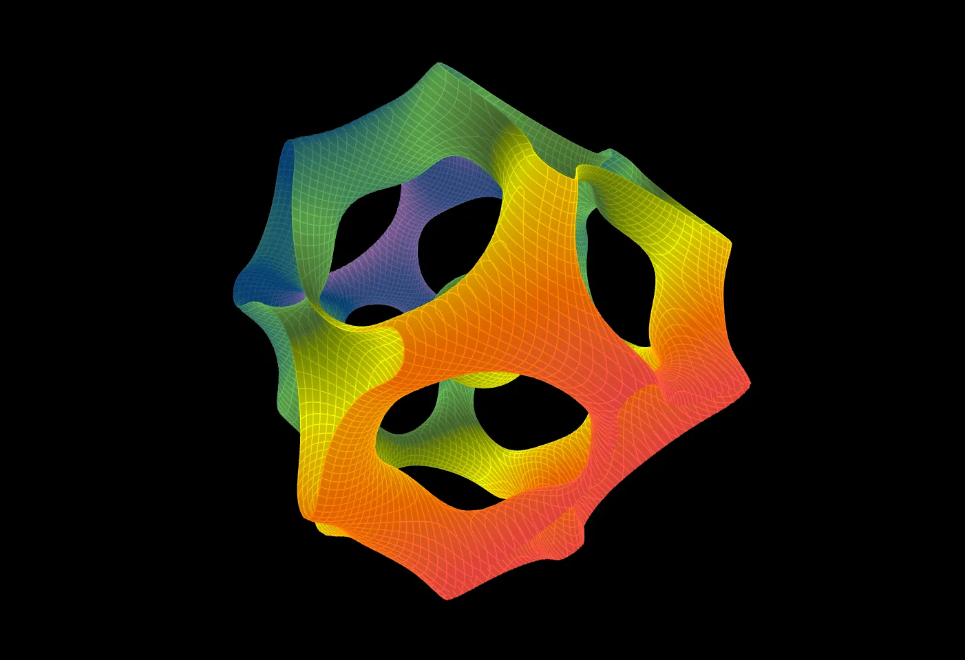
Bounds: -PI to PI, Resolution: 80

Chmutov Octic (This Guide's Example)

f(x,y,z) = x^8+y^8+z^8-2*x^6-2*y^6-2*z^6+1.25*x^4+1.25*y^4+1.25*z^4-0.25*x^2-0.25*y^2-0.25*z^2+0.03125
Bounds: -1 to 1, Resolution: 80
Backend: CPU, Render Mode: WIREFRAME

Klein Bottle

f(x,y,z) = (x*x + y*y + z*z + 2*y - 1) * ((x*x + y*y + z*z - 2*y - 1)^2 - 8*z*z) + 16*x*z*(x*x + y*y + z*z - 2*y - 1)
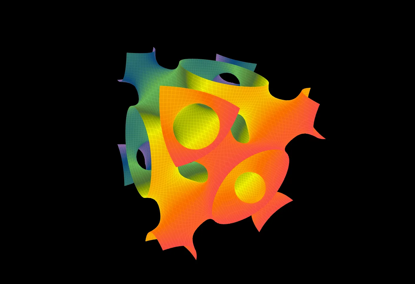
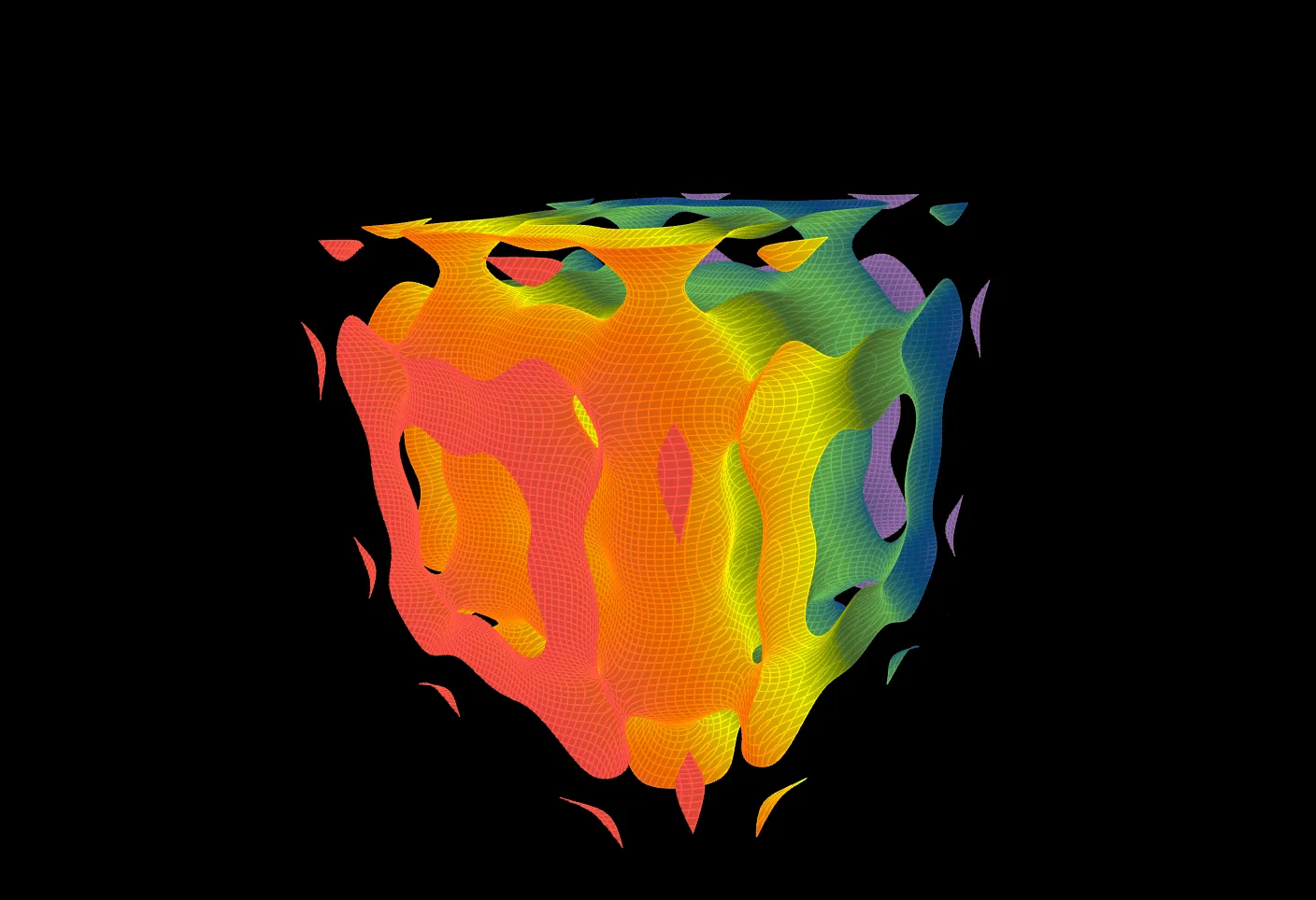
Bounds: -3 to 3, Resolution: 100

---

More Visual Examples

---

Technical Details

GPU Marching Cubes Rendering Pipeline

GPU mode uses OpenGL Compute Shaders for parallel Marching Cubes computation:

1. Voxel Evaluation Pass: Compute implicit function values at each voxel vertex in parallel using Compute Shaders
2. Triangle Generation Pass: Look up triangle configurations based on function values and generate all triangles in parallel
3. Rendering Pass: Render the triangle mesh using the Phong lighting model, supporting procedural textures

Shader Compilation

Implicit functions are compiled to GLSL shader code at runtime:

• FastExpressionParser parses the user-entered equation expression
• The parsed expression is compiled into GLSL code executable on the GPU
• Custom parameters are passed through uniform variables; modifying parameter values does not require shader recompilation
• Modifying the equation expression requires shader recompilation, which may cause brief stuttering

Parameter Animation Mechanism

ImplicitSurfaceParameterAnimator employs a sinusoidal oscillation + edge easing approach:

1. Sinusoidal Oscillation: Parameter values oscillate sinusoidally within [min, max]
2. Step Scaling: On start, step scale gradually increases from 0 to 1; on stop, it gradually decreases from the current value to 0
3. Edge Easing: Default configuration is attackRatio = 0.4, releaseRatio = 0.5, easing = SINE_OUT
4. Phase Synchronization: When starting animation, the initial phase is computed from the current parameter value, ensuring a smooth transition

---

Advanced Topics

Blending Formulas

Blending two implicit functions and :

• Union:
• Intersection:
• Difference:
• Smooth Blend: (k controls smoothness)

Understanding Chmutov Surfaces

Chmutov surfaces are algebraic surfaces based on Chebyshev polynomials , with the general form:

where is the n-th order Chebyshev polynomial. Chebyshev polynomials hold an important position in numerical analysis — they have the equioscillation property on the interval [-1, 1], which gives Chmutov surfaces their rich symmetry and singularity structures.

The Chmutov Octic surface uses the expanded form of the 8th-order Chebyshev polynomial, which is the equation in this guide's example. This surface possesses octahedral symmetry, presenting a complex and beautiful geometric structure.

Creating Custom Implicit Surfaces

1. Start with simple spheres or ellipsoids
2. Add parameters to control key shape features
3. Use min/max functions to combine multiple basic shapes
4. Use trigonometric functions to create periodic structures (like Gyroid)
5. Explore continuous changes in parameter space through parameter animation

---

Important Notes

1. Equation Validity:

   • Not all equations produce valid implicit surfaces
   • Some equations have no solution within the given range, resulting in an empty scene
   • Avoid division by zero (e.g., x/y when y might be 0) and square roots of negative numbers (e.g., sqrt(x) when x might be negative)

2. GPU Video Memory:

   • High resolution consumes significant GPU video memory
   • In GPU mode, voxel data needs to be allocated in video memory
   • If you encounter out-of-memory errors, reduce resolution or switch to CPU mode

3. Equation Modification:

   • Modifying the equation expression requires shader recompilation
   • Brief stuttering during recompilation is normal behavior
   • Modifying custom parameter values does not require recompilation and can be updated in real-time

4. Render Mode Limitations:

   • GPU backend only supports WIREFRAME render mode
   • To use PREVIEW (point cloud) mode, switch to CPU backend
   • Material and texture properties are only available in GPU + WIREFRAME mode

5. Sampling Range vs. Resolution Relationship:

   • Sampling range determines the visible area of the surface
   • Resolution determines the precision within the given range
   • At the same resolution, a larger sampling range means coarser precision

---

References

Mathematical Theory

• Lorensen, W.E. & Cline, H.E. - Marching Cubes: A High Resolution 3D Surface Construction Algorithm (SIGGRAPH 1987)
• Bloomenthal, J. - Polygonization of Implicit Surfaces (Computer-Aided Geometric Design, 1988)
• Hart, J.C. - Ray Tracing Implicit Surfaces (SIGGRAPH Course Notes, 1993)

Online Resources

• Wikipedia: Implicit Surface
• Wikipedia: Marching Cubes
• Wikipedia: Metaballs
• Wikipedia: Chebyshev polynomials
• MathWorld: Implicit Surface

Software Documentation

• OpenGL Compute Shader Programming Guide
• GLSL Language Specification