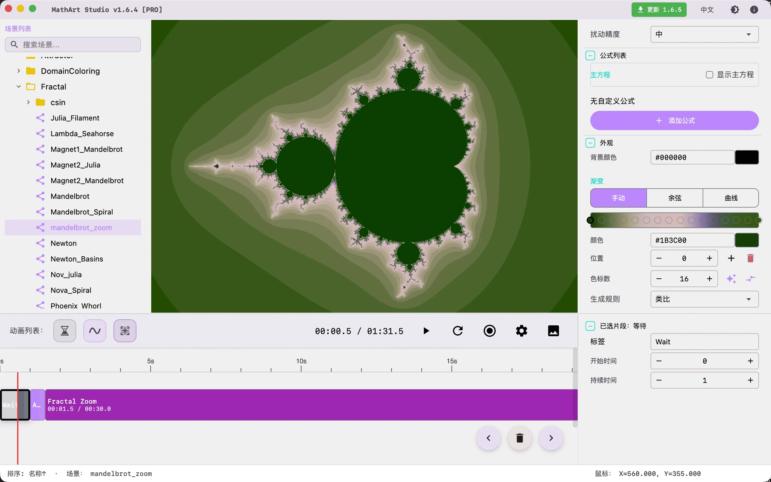
Fractal Scene
📖 Introduction
Fractals are one of the most core and powerful scenes in MathArt, allowing you to explore and create stunning mathematical art. A fractal is a geometric shape with self-similarity — no matter how much you zoom in, you'll see patterns similar to the whole. This "infinite nesting" property makes fractals one of the most fascinating domains where mathematics and art intersect.
This scene is powered by GPU Fragment Shader for high-performance rendering, supporting 10 built-in fractal formulas, 10 professional coloring algorithms, 3 gradient palette modes, and perturbation-based ultra-high-precision deep zooming. From the classic Mandelbrot set to the unique Spiral Septagon, each formula embodies profound mathematical beauty.
Note:
Symmetry Chaosis an independent scene pipeline and does not belong to the fractal formula panel on this page. To create web-style symmetric chaos images (such as Mercedes/Shield/Sunflower), please use theSymmetryChaos_*scene with its dedicated parameters and runtime settings.
Key Capabilities:
- High-Performance GPU Rendering: Pure GPU Fragment Shader rendering with three rendering strategies (Guessing/Multi Pass/One Pass) for real-time interactive exploration
- 10 Built-in Formulas: Covering power, Newton, rational, and transcendental kernel families — from classic to advanced
- 10 Coloring Algorithms: Including smooth coloring, decomposition, distance estimation, orbit trap, and other professional algorithms
- Perturbation Deep Zoom: DoubleDouble double-precision reference orbit computation, supporting Ultra-level precision down to 10⁻⁸ scale
- Triple Palette System: Manual palette, IQ cosine palette, and curve palette, combined with RGB/HSV color space interpolation
- Full Animation Support: Parameter oscillation animation, zoom keyframe animation, gradient offset animation, with timeline orchestration
🧮 Mathematical Background
What Are Fractals?
The term "fractal" was coined by mathematician Benoît B. Mandelbrot in 1975 in his book Les Objets Fractals, derived from the Latin fractus (broken). The most distinctive feature of fractals is self-similarity: the structure of the whole repeats itself in similar forms at any scale.
In complex dynamical systems, fractals are generated through iterative maps. By treating each point on the complex plane as an initial value and repeatedly applying the same mapping function, the complex plane is divided into different regions based on iteration behavior:
- Escape Set: Points that tend toward infinity after iteration, forming the exterior of the fractal
- Convergent Set: Points that converge to finite values (fixed points or periodic orbits) after iteration, forming the interior of the fractal
- Julia Set: The boundary between the escape set and the convergent set, possessing infinitely complex fractal structure
The Mandelbrot Set and Julia Sets
The Mandelbrot set is the most famous object in the study of complex dynamical systems, first rendered by computer by Benoît Mandelbrot in 1980. Its iteration formula is:
where is the iteration variable, is a parameter point on the complex plane, and is the power (classically 2). The Mandelbrot set studies parameter space: for each parameter , it determines whether the iteration starting from escapes.
Julia sets are closely related to the Mandelbrot set, independently studied by French mathematicians Gaston Julia and Pierre Fatou in 1918-1919. Julia sets use the same iteration formula but study dynamical space: the parameter is fixed, and for different initial values , it determines whether the iteration escapes.
There is a profound duality between the Mandelbrot set and Julia sets: each point in the Mandelbrot set corresponds to a Julia set. When lies inside the Mandelbrot set, the corresponding Julia set is connected; when lies outside the Mandelbrot set, the corresponding Julia set is totally disconnected (Cantor dust).
Newton Fractals
Newton fractals are based on Newton's root-finding method. For the equation , the Newton iteration is:
where is the relaxation factor, defaulting to 1. Different initial values converge to different roots of the equation, and the partition of convergence boundaries produces beautiful fractal patterns. Unlike escape-type fractals, Newton fractals use convergence criteria rather than escape criteria.
Historical Background
The development of fractal theory spans the 20th century history of mathematics:
- 1918-1919: Gaston Julia and Pierre Fatou independently studied the dynamical behavior of complex iterative functions, laying the theoretical foundation for Julia sets
- 1920s-1970s: Fractal theory remained at the margins of mathematics, as its complex structures were difficult to study with traditional methods
- 1975: Benoît Mandelbrot coined the term "fractal" and first rendered the Mandelbrot set by computer in 1980
- 1980s: Advances in computer graphics made fractal visualization possible, and fractal art began to flourish
- 2000s: The introduction of perturbation theory made deep zooming a reality, with Karl Runmo and others achieving zoom levels of 10⁻¹⁰⁰⁰
🖥️ Interface Overview
All controls are located in the inspector panel on the right, divided into six main sections:
- Geometry: Select fractal formulas, variants, adjust formula parameters, view controls, and render settings
- Camera: Control viewing angles
- Formulas: Display mathematical formulas and annotations
- Appearance: Adjust background color, gradient palettes, coloring algorithms, and coloring parameters
- Parameters: Define custom constants used in equations (advanced usage)
- Animation: Timeline and animation controls
⚙️ Configuration Guide
1. Geometry (Geometry Settings)
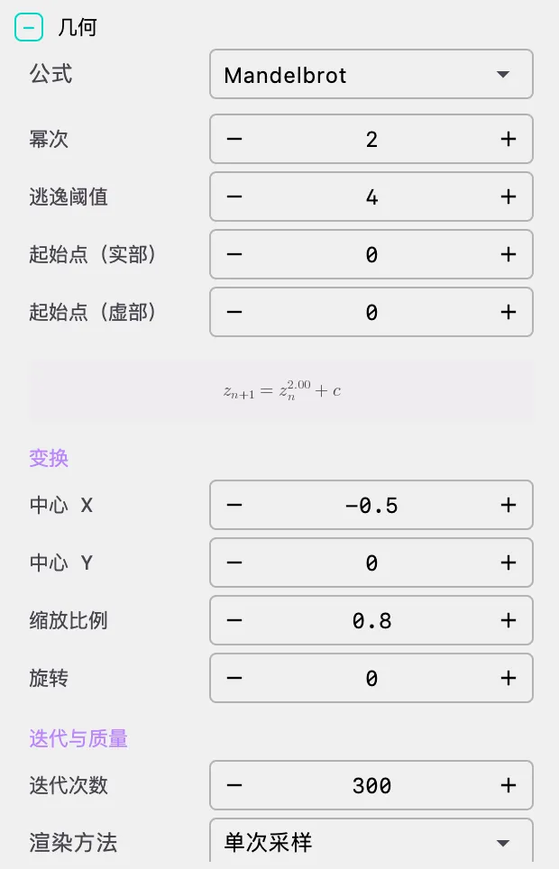
Geometry settings are the core of the Fractal scene, determining the basic form, mathematical characteristics, and rendering method of the fractal.
Formula Selection
The system provides 10 built-in fractal formulas, categorized by kernel family:
Power Kernel Family (POWER)
Mandelbrot
- The most classic fractal pattern, displaying infinite details on the complex plane
- Iteration formula:
- Parameters: power, bailout, start_point
- Supported variants: Mandelbrot / Julia
- Supports perturbation: Yes
- Termination policy: Escape
Julia
- Closely related to Mandelbrot, each Julia set corresponds to a point in the Mandelbrot set
- Iteration formula: , where is a fixed Julia seed value
- Parameters: power, bailout, start_point, julia_seed
- Supports perturbation: Yes
- Termination policy: Escape
Mandelbrot and Julia share the same iteration formula; the difference lies in the role of parameter : in Mandelbrot, is a variable on the complex plane, while in Julia, is a fixed constant.
Newton Kernel Family (NEWTON_GENERIC)
Newton
- Based on Newton's root-finding algorithm, showing beautiful patterns of mathematical equation solving
- Iteration formula:
- Parameters: exponent (supports complex values), relaxation
- Supports perturbation: Yes
- Termination policy: Convergence
- Note: Newton fractal uses convergence criteria rather than escape criteria; coloring parameter settings differ from other fractals
Nova
- A variant of Newton fractal that introduces an additional term in the Newton iteration
- Iteration formula:
- Parameters: exponent (supports complex values), relaxation, start_value
- Supported variants: Mandelbrot / Julia
- Supports perturbation: Yes
- Termination policy: Convergence
Rational Kernel Family (RATIONAL)
Phoenix
- Has a flame-like appearance with rich color layers
- Uses the previous iteration value in calculation, producing unique feedback effects
- Parameters: exponent1, exponent2, distortion
- Does not support perturbation; precision is limited during deep zooming
- Termination policy: Escape
Magnet I & II
- Includes Magnet I and Magnet II, shaped like magnetic attraction
- Based on rational function iteration, with both escape and convergence characteristics
- Parameters: perturbation, parameter, convergent_bailout
- Does not support perturbation
- Termination policy: Hybrid; requires both escape and convergence thresholds
Lambda
- Displays the complex structure of parameter space
- Based on complex logistic map:
- Parameters: lambda coefficient
- Does not support perturbation
- Termination policy: Escape
Spiral Septagon
- Unique fractal with spiral and septagon features
- Based on rational function iteration, requires singularity guard parameter
- Parameters: Phi, exponent, singularity_guard
- Does not support perturbation
- Termination policy: Escape
- Note: The singularity guard threshold prevents numerical calculation anomalies; it is recommended not to modify the default value
Transcendental Kernel Family (TRANSCENDENTAL)
Complex Sin
- Fractal based on complex sine function
- Iteration formula:
- Produces unique transcendental function fractal patterns
- Does not support perturbation
- Termination policy: Escape
[Screenshot placeholder: Showing comparison of different formula fractal effects]
Variant Selection
Some fractal formulas support both Mandelbrot and Julia variants:
- Mandelbrot Variant: Explores parameter space on the complex plane, each point corresponds to a Julia set
- Julia Variant: Uses fixed Julia seed values, displaying the Julia set pattern for that seed
When a formula supports both variants, you can switch between them using the "Variant" dropdown menu. Currently, formulas supporting dual variants include: Mandelbrot, Nova.
When switching variants, the system automatically synchronizes formula parameters. When switching from Mandelbrot to Julia, the current Julia constant is activated as the iteration parameter.
Formula Parameters
Each fractal formula has its specific parameters that directly affect the fractal's form. The parameter panel is dynamically generated based on formula metadata, supporting the following parameter types:
- Integer parameters: Such as power, symmetry degree, etc., using stepper input
- Float parameters: Such as bailout, relaxation, etc., using numeric input
- Complex parameters: Such as julia_seed, exponent, etc., split into real (Re) and imaginary (Im) components
- Boolean parameters: Using toggle switches
Common Parameter Reference
| Parameter | Meaning | Type | Default | Description |
|---|---|---|---|---|
| power | Power | Integer/Complex | 2 | Controls the basic form of the fractal; p=2 is the classic form |
| bailout | Bailout radius | Float | 4.0 | Threshold for determining if a point escapes |
| start_point | Start point | Complex | (0, 0) | Iteration starting point |
| julia_seed | Julia seed | Complex | Varies | Defines the form of the Julia set |
| relaxation | Relaxation factor | Float | 1.0 | Convergence speed control for Newton/Nova |
| exponent | Exponent | Complex | Varies | Equation power for Newton/Nova |
| convergent_bailout | Convergent bailout | Float | 1e-6 | Convergence judgment threshold for Magnet |
Tip: Click on a point in the Mandelbrot set to quickly set that point as the Julia seed — this is the most intuitive way to explore Julia sets.
View Controls
- Center X/Y: Defines the center coordinates of the view, supports high-precision display (DoubleDouble double precision), suitable for deep zooming
- Zoom: Controls the magnification of the view; larger values reveal more details; can quickly adjust with mouse scroll wheel
- Rotation: Controls the rotation angle of the view (radians); can create rotation animation effects
Note: Deep zooming (Zoom > 100) requires enabling the perturbation algorithm to maintain precision. Center coordinates use DoubleDouble double-precision representation, accurate to 10⁻³⁰ scale.
Render Settings
Render Method
MathArt provides three rendering methods that balance quality and performance:
| Render Method | Characteristics | Use Case |
|---|---|---|
| Guessing | Uses smart algorithm to predict details, fastest rendering | Quick preview, parameter exploration |
| Multi Pass | Renders lower resolution first, then progressively increases | Interactive exploration |
| One Pass | Renders full resolution in one go, highest quality | Final output |
Recommendation: Use Guessing or Multi Pass during exploration, switch to One Pass for final output to get the best quality.
Perturbation Precision
Perturbation algorithm is an advanced rendering technique allowing ultra-high precision fractal rendering. When the zoom level exceeds a threshold, the system automatically enables the perturbation algorithm:
| Precision Level | Threshold | Description |
|---|---|---|
| Low | 1.0e-2 | Fast rendering, lower precision, suitable for quick preview |
| Medium | 1.0e-4 | Balanced precision and speed, suitable for most cases |
| High | 1.0e-6 | High precision rendering, suitable for moderate deep zooming |
| Ultra | 1.0e-8 | Highest precision, suitable for deep zooming, but requires more computational resources |
Perturbation Algorithm Support:
| Formula | Supports Perturbation | Reason |
|---|---|---|
| Mandelbrot | ✅ | Integer power, meets perturbation conditions |
| Julia | ✅ | Integer power, meets perturbation conditions |
| Newton | ✅ | Meets perturbation conditions |
| Nova | ✅ | Meets perturbation conditions |
| Phoenix | ❌ | Iteration depends on previous value, doesn't meet perturbation conditions |
| Magnet I/II | ❌ | Rational function iteration, doesn't meet perturbation conditions |
| Lambda | ❌ | Doesn't meet perturbation conditions |
| Complex Sin | ❌ | Transcendental function, doesn't meet perturbation conditions |
| Spiral Septagon | ❌ | Rational function, doesn't meet perturbation conditions |
2. Camera (Camera Control)
Adjust viewing angles and camera parameters. The Fractal scene is always rendered in 2D; camera controls are primarily used for rotation and tilted viewing.
- Phi (Pitch Angle): Vertical angle of the camera, range 0 to π, default π/2 (horizontal view)
- Theta (Yaw Angle): Horizontal angle of the camera, range 0 to 2π, default 0
- Gamma (Roll Angle): Rotation angle of the camera, range 0 to 2π, default 0
Fractals are typically viewed from directly above (Phi = 0 or π) or horizontally (Phi = π/2). Camera rotation animations can be created with the timeline system.
3. Formulas (Formula Display)
Display mathematical formulas and equations in the scene, perfect for creating educational videos or showcasing the mathematical beauty of fractals.
Main Equation Display
- Show Main Equation: Toggle main equation display on/off
- The system automatically generates formula text based on the current formula and parameters
- Main Equation Position:
- X: Horizontal position coordinate
- Y: Vertical position coordinate
- Scale: Formula scaling ratio
- Color: Formula color
Custom Formulas
Add multiple custom formulas to the scene:
- Add Formula: Click "Add Formula" button to add a new formula
- Formula Content: LaTeX format, X/Y position, scale, color
- Delete Formula: Click the delete button in the top-right corner of the formula to remove it
4. Appearance (Appearance Settings)
Appearance settings give you complete control over the fractal's visual presentation, from colors to coloring algorithms, creating unique artistic works.
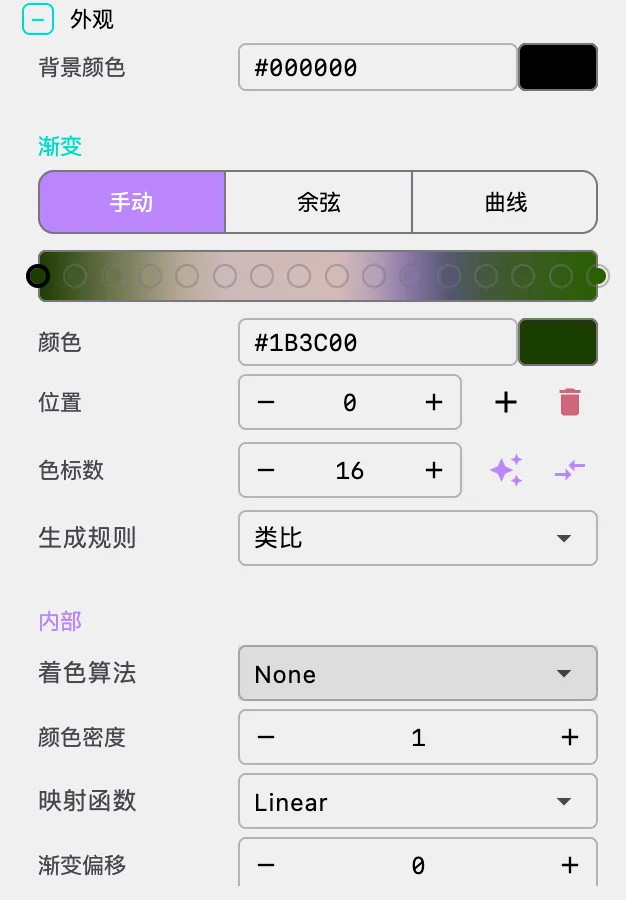
Background Color
- Background Color: Set the rendering background color
- Fractals typically use black or dark backgrounds to highlight details
Gradient Palette
Gradient (color mapping) is the core of fractal art, determining the fractal's color presentation. MathArt provides three gradient modes:
Manual Palette Mode
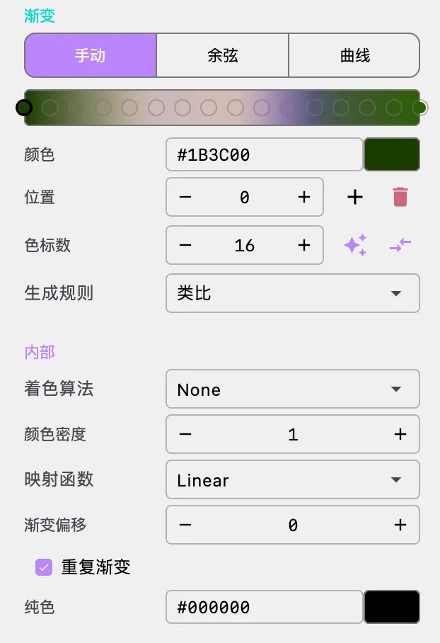
Manual palette lets you precisely control each color stop:
- Color Stops: Supports up to 25 color stops
- Add Color: Click the "+" button below the palette to add a new color
- Delete Color: Double-click a color stop to delete it (minimum 2 colors required)
- Adjust Color: Click a color block to open the color picker
- Adjust Position: Drag color stops to change their position in the gradient
- Random Generation: Click the random button to generate a random palette
- Reverse: Click the reverse button to reverse color order
Random Palette Strategies:
| Strategy | Characteristics |
|---|---|
| Monochromatic | Variations based on a single hue |
| Analogous | Uses adjacent hues |
| Complementary | Uses contrasting hues |
| Split Complementary | Uses split complementary hues |
Tips: Use high-contrast colors to highlight fractal details; adjacent colors with similar tones create smooth transitions; warm-cool color contrasts often produce stunning effects.
Cosine Palette Mode
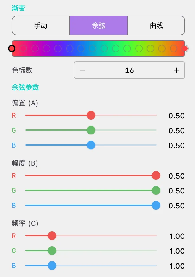
Cosine palette generates smooth gradient effects using the IQ (Inigo Quilez) mathematical formula:
| Parameter | Meaning | Effect |
|---|---|---|
| Bias (A) | Base color value | Controls the baseline value of color channels |
| Amplitude (B) | Color variation amplitude | Controls the range of color channel variation |
| Frequency (C) | Color variation frequency | Controls the number of color cycles |
| Phase (D) | Color variation starting phase | Controls the starting position of color cycles |
Each parameter can be adjusted separately for red, green, and blue color channels.
Cosine palette is especially suitable for creating rainbow-like smooth color transitions. Adjusting frequency controls the density of color cycles; use the random button to quickly generate beautiful palettes.
Curve Palette Mode
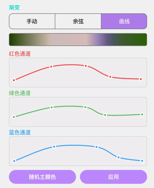
Curve palette provides the most flexible color control, using editable Bézier curves to separately control R/G/B channels:
- Add Control Point: Click on an empty area of the curve to add a new control point
- Delete Control Point: Double-click a control point to delete it (minimum 2 points required)
- Move Control Point: Drag control points to adjust curve shape
- Channel Switching: Edit red, green, and blue color channels separately
Use S-curves for smooth color transitions; try different curve shapes for different channels to create unique color effects.
Palette Space
Choose the color space for color interpolation:
- RGB: Interpolate in RGB color space, direct color transitions
- HSV: Interpolate in HSV color space, more natural and harmonious color transitions
HSV space typically produces more harmonious color transition effects, recommended for most cases.
Coloring Algorithm
The coloring algorithm determines how iteration results are mapped to colors. MathArt provides 10 professional coloring algorithms, divided into index-type (INDEX) and direct-type (DIRECT) categories:
[Screenshot placeholder: Showing comparison of different coloring algorithm effects]
Inside Coloring
Inside coloring applies to points inside the fractal set (non-escaping/converging points):
| Algorithm | Output Type | Description |
|---|---|---|
| None | INDEX | Use solid fill color |
| Basic | INDEX | Simple coloring based on iteration count, supports multiple metrics |
| Smooth Mandelbrot | INDEX | Produces smooth color transitions, eliminates banding |
| Decomposition | INDEX | Angle-based coloring, shows complex phase information |
| Binary Decomposition | INDEX | Sign-based binary coloring |
| Distance Estimator | INDEX | Coloring based on distance to set boundary |
| Direct Domain | DIRECT | Use complex values directly as colors |
| Direct Orbit Trap | DIRECT | Coloring based on orbit traps |
| Direct Normalized Z | DIRECT | Normalized complex value coloring |
| Orbit Trap (Index) | INDEX | Index-based orbit trap coloring |
Outside Coloring
Outside coloring applies to points outside the fractal set (escaping points), providing the same algorithm options as inside coloring, but typically with different parameter settings.
For Mandelbrot/Julia sets, outside coloring is usually more important than inside coloring. Smooth Mandelbrot is the most commonly used outside coloring algorithm for smooth color transitions.
Coloring Parameters
Each coloring algorithm has its specific parameters, divided into common parameters and algorithm-specific parameters:
Common Parameters
Color Density
- Controls the frequency of color variation
- Larger values create more color cycles
- Recommended range: 0.1 - 10.0
Transfer Function
Controls the mapping from iteration values to color indices:
| Transfer Function | Mathematical Expression | Effect |
|---|---|---|
| None | Use raw values directly | |
| Linear | Linear mapping | |
| SQR | Enhances high-value areas | |
| SQRT | Enhances low-value areas | |
| CUBE | Strongly enhances high-value areas | |
| CUBEROOT | Strongly enhances low-value areas | |
| LOG | Compresses high-value areas, reveals more detail | |
| EXP | Expands high-value areas | |
| SIN | Creates periodic variations | |
| ARCTAN | Smooth transitions |
Tips: Using LOG transfer function reveals more details; SQR and CUBE are good for highlighting main fractal structures; SQRT and CUBEROOT are good for revealing fine details.
Gradient Offset
- Adjusts the starting position of colors in the gradient
- Used for fine-tuning color distribution
Repeat Gradient
- Checked: Colors cycle repeatedly
- Unchecked: Use solid color for out-of-range areas
Solid Color
- The color used for out-of-range areas when not repeating gradient
Algorithm-Specific Parameters
Basic Coloring
- Metric: Select the metric to use for coloring
- ITERATION: Iteration count
- REAL: Real part value
- IMAGINARY: Imaginary part value
- SUM: Sum of real and imaginary parts
Smooth Mandelbrot Coloring
- Exponent: Usually same as fractal's power, supports complex values
- Power: Affects smoothness
- Bailout: Should match the fractal's bailout setting
Binary Decomposition Coloring
- Decomposition Type:
- TYPE_1: Based on real part sign
- TYPE_2: Based on imaginary part sign
Distance Estimator Coloring
- Power: Should match the fractal's power
Direct Domain Coloring
- Scale: Color scaling factor
- Gamma: Gamma correction value
- Saturation: Color saturation
Direct Orbit Trap Coloring
- Trap Shape: Point, ring, cross
- Trap Radius: Trap size
- Trap Center: Trap position
- Rotation: Trap rotation angle
- Aspect Ratio: Trap shape proportion
- Threshold: Trap activation threshold
- Mix Factor: Gradient mixing ratio
- Merge Opacity: Orbit merge transparency
5. Parameters
Define custom constants used in equations, which is an advanced usage. In most cases, the formula parameter panel already provides all necessary parameter controls.
🎬 Animation and Timeline
The Fractal scene supports powerful animation features, allowing you to create dynamic fractal art.
Parameter Oscillation Animation
Parameter oscillation animation is implemented through FractalParameterAnimator, allowing parameters to undergo periodic sinusoidal oscillation within a specified range.
How It Works
- For each parameter, specify the oscillation step, range (min, max), and edge easing
- The parameter value oscillates sinusoidally within [min, max]:
value = mid + amp * sin(phase) - Oscillation speed is jointly controlled by the step and step scale factor
- Edge easing ensures the parameter decelerates near range boundaries, avoiding abrupt changes
Animatable Parameters
All formula parameters support animation, including:
- View Parameters: Center X/Y, Zoom, Rotation
- Iteration Parameters: Iterations, Bailout
- Julia Parameters: Julia Cx/Cy
- Formula-Specific Parameters: Dynamically determined based on formula type
Parameter Modes
The animator supports four parameter modes:
- SCALAR: Scalar parameters, such as iteration count, bailout radius
- COMPLEX_FULL: Complex parameters, both real and imaginary parts oscillate simultaneously
- COMPLEX_REAL: Complex parameters, only real part oscillates
- COMPLEX_IMAG: Complex parameters, only imaginary part oscillates
Zoom Animation
Create stunning zoom animations — the most distinctive animation type for the Fractal scene:
Features:
- Supports high-precision coordinates, can create deep zoom animations
- Uses logarithmic interpolation for more natural zoom changes
- Supports zoom-aware center point movement
Creating Zoom Animation:
- Add a zoom animation clip
- Set start and end zoom levels
- Set target center position
- Adjust animation curve to control zoom speed
Tip: Using exponential zoom curves creates more natural zoom effects; enable high-precision perturbation for deep zooming.
Gradient Animation
Gradient animation makes colors change over time:
- Palette Offset: Shift the overall palette position
- Inside Gradient Offset: Shift the gradient for inside coloring
- Outside Gradient Offset: Shift the gradient for outside coloring
Configuration Method
Define animation sequences through the timeline array in JSON configuration:
{
  "timeline": [
    {
      "type": "wait",
      "duration": 5,
      "label": "Wait",
      "easing": "SINE_IN_OUT"
    }
  ]
}
[Screenshot placeholder: Showing timeline panel and animation settings]
🚀 Performance & Best Practices
Recommended Configurations
| Goal | Iterations | Render Method | Perturbation Precision | Coloring Algorithm |
|---|---|---|---|---|
| Quick Exploration | 100-300 | Guessing | Low/Medium | Basic |
| Interactive Adjustment | 300-500 | Multi Pass | Medium/High | Smooth Mandelbrot |
| High Quality Output | 500-2000 | One Pass | High/Ultra | Smooth Mandelbrot / DE |
| Deep Zoom | 1000+ | One Pass | Ultra | Smooth Mandelbrot |
Performance Optimization Tips
Iterations:
- Use lower values during exploration (100-300), increase after finding a satisfactory composition
- Iteration count has an approximately linear relationship with rendering time
Render Method:
- Use Multi Pass for interaction, One Pass for output
- Guessing is fastest but may lose details
Coloring Algorithm:
- Basic coloring renders fastest
- Direct series algorithms require additional computation, rendering slightly slower
- Distance Estimator requires derivative computation, rendering slowest
Perturbation Algorithm:
- Automatically enables only during deep zooming
- Higher precision levels require more computational resources and memory
- Formulas that don't support perturbation will experience precision loss during deep zooming
Palettes:
- Manual and cosine palettes have the same rendering efficiency
- Gradient LUT is pre-computed on the CPU side, with minimal impact on rendering performance
❓ Troubleshooting
Fractal Looks Blurry
Problem: Rendered result is blurry, details are unclear
Cause: Insufficient iterations or precision loss from excessive zoom level
Solutions:
- Increase iteration count (recommended 300+)
- Use perturbation algorithm to improve precision (High or Ultra)
- Check render method settings; One Pass has the highest quality
- Confirm bailout radius is set reasonably (typically 4.0)
Visible Color Banding
Problem: Fractal colors show stripe-like banding, not smooth enough
Cause: Improper coloring algorithm or transfer function selection
Solutions:
- Use Smooth Mandelbrot coloring algorithm instead of Basic
- Choose LOG or SQRT transfer function
- Use HSV palette space
- Try cosine or curve palette modes
Rendering Too Slow
Problem: Fractal rendering takes too long
Cause: Parameters set too high or improper render method
Solutions:
- Reduce iteration count
- Use Guessing or Multi Pass render method
- Simplify coloring algorithm (Basic is fastest)
- Lower perturbation precision (if deep zooming is not needed)
- Disable perturbation algorithm (not needed for shallow zooming)
Pixelation During Deep Zoom
Problem: Image shows block-like pixels after deep zooming
Cause: Insufficient floating-point precision; standard double precision exhausts its precision after zooming beyond 10¹³ times
Solutions:
- Ensure using a formula that supports perturbation (Mandelbrot, Julia, Newton, Nova)
- Set perturbation precision to High or Ultra
- For formulas that don't support perturbation, deep zoom precision limitation is an inherent mathematical constraint
How to Find Interesting Fractal Details
Suggestions:
- Start exploring from the Mandelbrot set
- Zoom into boundary areas — the richest details are always on the boundary
- Look for spirals, seahorses, elephant trunks, and other classic structures
- Use different coloring algorithms to highlight details
- Try different formula and parameter combinations
- Adjust color density and transfer function to change visual presentation
How to Create Julia Sets
Steps:
- Select a formula that supports Julia variant (like Mandelbrot, Nova)
- Select "Julia" from the variant dropdown menu
- Adjust the Julia seed parameter
- Tip: Click on a point in the Mandelbrot set to quickly set that point as the Julia seed
📐 Classic Fractal Examples
Mandelbrot Set (Default Configuration)
The following is MathArt's built-in Mandelbrot example configuration (mandelbrot.json):
Formula: Mandelbrot
Variant: MANDELBROT
Power: 2
Bailout: 4
Iterations: 300
Center: (-0.7, 0)
Zoom: 0.5
Rotation: 0
Render Method: Multi Pass
Perturbation Precision: Ultra
Palette (16 colors):
#2A2A32 → #304A58 → #376B7E → #3E8CA4 → #52ACB6 → #8AB5BC → #C2BEC2 → #CCC79A
→ #D4B75B → #DB8F1C → #B86707 → #753F0C → #332211 → #251915 → #17111A → #10081F
Coloring Configuration:
Outside Coloring: Basic (Metric=ITERATION, Color Density=3, Transfer Function=LINEAR)
Inside Coloring: None (Solid Color=#000000)
Julia Set (Near Seahorse Valley)
Formula: Mandelbrot
Variant: JULIA
Power: 2
Julia Seed: (-0.8123, 0.016)
Bailout: 4
Iterations: 500
Newton Fractal (Three Roots)
Formula: Newton
Exponent: 3 (real)
Relaxation: 1.0
Iterations: 200
Nova Fractal (Five Roots)
Formula: Nova
Variant: MANDELBROT
Exponent: 5 (real)
Relaxation: 1.0
Start Value: (1, 0)
Iterations: 300
🔧 Technical Details
GPU Rendering Pipeline
The Fractal scene uses a GPU Fragment Shader rendering pipeline with the following core workflow:
Shader Compilation:
ShaderCompilationManagerdynamically compiles Fragment Shaders based on formula registration information- Uses a part-concatenation architecture: 22 GLSL parts are concatenated as needed, with
#definemacros injected - Compilation results are cached to avoid recompilation
Render Execution:
- Set all uniforms (center, zoom, rotation, iterations, formula parameters, coloring parameters)
- Determine whether to enable perturbation algorithm
- If perturbation is needed: compute reference orbit → pack RGBA32F texture → upload to GPU
- Generate Gradient LUT texture (1024 sample points)
- Draw full-screen QUAD; Fragment Shader computes per-pixel
Coloring Pipeline:
- Fragment Shader executes formula iteration
- Calculates color index or direct color based on coloring algorithm
- Samples final color through Gradient LUT or Cosine Palette
Perturbation Algorithm
Perturbation theory is the core technology for deep zooming, proposed by Pauldelbrot and others in 2013-2014 on the fractalforums.com community:
Working Principle:
- Compute the complete orbit of a reference point using DoubleDouble double precision on the CPU
- Upload the reference orbit as an RGBA32F texture to the GPU
- For each pixel on the GPU, perform perturbation iteration based on the reference orbit
- Avoids precision loss from standard double-precision floating-point during deep zooming
Precision Determination:
- The formula must support perturbation (meeting specific mathematical conditions)
- The power must be an integer
- The zoom level must exceed the threshold (zoom > 100)
- Iteration count > 0
Formula Registration System
The formula system uses a registry-driven plugin architecture:
FormulaRegistry: Global formula registry (ConcurrentHashMap), singleton patternFormulaMetadata: Describes the complete capabilities and parameters of formulas; UI layer auto-generates editors based on thisStandardFormulaCatalog: Registers 10 built-in formulasFormulaDomainService: Builds runtime state, evaluates perturbation availability, packs parameters
Coloring Algorithm Registration System
The coloring algorithm system also uses a registry pattern:
ColoringRegistry: Global coloring algorithm registryColoringMetadata: Describes output type, applicable domain, and parameter definitions of coloring algorithmsStandardColoringCatalog: Registers 10 built-in coloring algorithmsColoringRuntimeMapper: Resolves request IDs, validates parameters, returns mapping results
Triple Color System
- Palette Direct Transfer: Up to 16-color palette passed as
u_paletteuniform to shader - Cosine Palette: IQ-style cosine palette, parameters a/b/c/d passed through uniforms
- Gradient LUT: CPU pre-computes 1024-point lookup table, uploaded as RGB32F texture to GPU, supports RGB/HSV interpolation
🎨 Creative Techniques
Parameter Exploration
- Start from Classic Formulas: Mandelbrot is the best starting point; boundary regions contain infinite details
- Zoom into Boundaries: The richest details of fractals are always at the boundary between escape and convergent sets
- Adjust Power: Changing the power creates different morphological variants; p=3 produces three-fold symmetry
- Explore Julia Sets: Selecting Julia seeds near the Mandelbrot set boundary often reveals exquisite patterns
Visual Tuning
Coloring Schemes:
- First select an appropriate coloring algorithm (Smooth Mandelbrot is the most versatile choice)
- Then adjust the transfer function (LOG for revealing details, SQR for highlighting structure)
- Finally fine-tune color density and gradient offset
Color Combinations:
- Use cosine palette to quickly generate harmonious color schemes
- Dark backgrounds with high-saturation colors typically produce the best results
- HSV color space interpolation is usually more harmonious than RGB
Detail Enhancement:
- Distance Estimator coloring clearly reveals fractal boundaries
- Increasing color density reveals more layers
- Orbit Trap coloring creates unique artistic effects
Animation Design
Zoom Animation:
- This is the most distinctive animation type for fractals
- Select an interesting target point, set start and end zoom levels
- Use exponential zoom curves for more natural zoom speed
- Always enable high-precision perturbation for deep zooming
Parameter Oscillation:
- Set oscillation animation for Julia seeds to observe pattern morphological evolution
- Set oscillation for power to create morphological transition effects
- Edge easing ensures smooth transitions at range boundaries
Gradient Animation:
- Gradient offset animation makes colors "flow"
- Combined with zoom animation, the effect is even more stunning
⚠️ Important Notes
Perturbation Algorithm Limitations:
- Not all formulas support the perturbation algorithm
- Phoenix, Magnet, Lambda, Complex Sin, and Spiral Septagon do not support perturbation
- Formulas that don't support perturbation have limited precision during deep zooming; this is an inherent mathematical constraint
Iteration Count and Quality:
- Too few iterations results in lost detail, manifesting as large areas of solid color
- Too many iterations significantly increases rendering time but may not bring visible improvement
- Recommended to start with lower values and gradually increase until detail no longer increases
Bailout Radius Settings:
- The bailout radius affects the sensitivity of escape detection
- A bailout radius that's too small may cause points that should escape to be misjudged as interior
- A bailout radius that's too large wastes iteration counts
- The classic Mandelbrot set bailout radius is typically set to 4.0 (i.e., |z|² > 4)
Newton/Nova Convergence Criteria:
- These two formulas use convergence criteria rather than escape criteria
- Inside coloring is more important for Newton/Nova
- Differences in convergence speed can produce rich color layers
Magnet Fractal Hybrid Termination Policy:
- Magnet formulas have both escape and convergence characteristics
- Both escape radius and convergence threshold need to be set
- The balance between the two thresholds significantly affects rendering results
💡 Advanced Topics
Understanding the Mathematical Principles of Perturbation
Standard double-precision floating-point numbers have approximately 15-16 significant digits. When the zoom level exceeds 10¹³ times, the distance between adjacent pixels becomes smaller than the floating-point precision, causing all pixels to compute the same iteration value — this is the cause of "pixelation."
The core idea of the perturbation algorithm is: select a reference point , compute its complete orbit with high precision, then for nearby points , compute the perturbation with standard precision:
Since is typically much smaller than , standard precision is sufficient to represent the significant digits of , thereby avoiding precision loss.
The Duality Between Mandelbrot and Julia Sets
The Mandelbrot set can be viewed as a "catalog" of Julia sets: for each point in the Mandelbrot set, there exists a corresponding Julia set . When lies inside the Mandelbrot set, is connected; when lies outside the Mandelbrot set, is totally disconnected (Cantor dust).
Points near the boundary of the Mandelbrot set correspond to the most complex and beautiful Julia sets. This is why selecting Julia seeds near the Mandelbrot set boundary often produces the most exquisite patterns.
Mathematical Principles of Coloring Algorithms
Smooth Mandelbrot coloring uses normalized iteration count to eliminate banding:
where is the iteration count at escape and is the power. This formula maps discrete iteration counts to continuous values, achieving smooth color transitions.
Distance Estimator coloring is based on distance estimation to the fractal set boundary:
where is the derivative of with respect to . Points with smaller distances are closer to the set boundary; rendering them with different brightness can highlight the fine structure of the boundary.
Creating Custom Fractal Patterns
Although MathArt uses preset formulas, you can create richly varied fractal patterns through clever parameter adjustment:
- Start from the classic Mandelbrot set, zoom into a boundary region of interest
- Switch to Julia variant, set the current view center as the Julia seed
- Fine-tune the real and imaginary parts of the Julia seed, observing subtle pattern changes
- Try different power values to explore non-classical forms
- Use Newton/Nova formulas, adjusting exponent and relaxation to create entirely new patterns
- Use parameter oscillation animation to explore continuous changes in parameter space
📚 References
Mathematical Theory
- Benoît B. Mandelbrot - The Fractal Geometry of Nature (1982)
- Gaston Julia - Mémoire sur l'itération des fonctions rationnelles (1918)
- Pierre Fatou - Sur les équations fonctionnelles (1919-1920)
- Heinz-Otto Peitgen & Peter H. Richter - The Beauty of Fractals (1986)
Online Resources
- Wikipedia: Mandelbrot Set
- Wikipedia: Julia Set
- Wikipedia: Newton Fractal
- Inigo Quilez - Cosine Palettes — Cosine palette formula reference
- Fractal Forums — Fractal enthusiast community
Perturbation Algorithm
- Pauldelbrot - Perturbation Theory for the Mandelbrot Set (2013-2014, fractalforums.com)
- Karl Runmo - Deep Zoom Technology — Achieved zoom levels of 10⁻¹⁰⁰⁰