Domain Coloring

Introduction

Domain Coloring Example

Domain Coloring is a classic method for visualizing complex-valued functions — it colors every point on the complex plane, allowing us to "see" the full picture of a function in the world of complex numbers. From Riemann's conformal mapping theory to modern fractal exploration, domain coloring transforms abstract complex analysis into an intuitive visual experience, making core concepts such as zeros, poles, and branch points immediately recognizable.

Key Capabilities:

Free Formula Input: Supports 25 complex functions; enter any complex function expression and it is compiled to a GPU shader in real time
Iterative Fractal System: Built-in three seed modes (Mandelbrot style, Julia style, Newton style) with custom iteration formulas
Level Curve Visualization: Four level curve modes (Phase, Modulus, Phase+Modulus, None) with fine-grained control over stripe density and sharpness
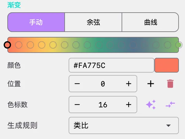
Palette System: Supports manual, cosine, and curve gradient modes, combined with JSON palettes for rich color expression
Full Animation Support: Parameter oscillation animation, domain rotation animation, and gradient animation, with edge easing for smooth transitions
GPU/CPU Dual-Path Rendering: GPU-first with automatic CPU fallback for compatibility

Mathematical Background

What is Domain Coloring?

A complex-valued function f(z) maps one complex number z to another complex number w = f(z). Unlike real-valued functions, the graph of a complex function cannot be directly plotted on a two-dimensional plane — because both input and output are two-dimensional. Domain coloring solves this problem by coloring each point z on the complex plane: the color encodes information about f(z).

Specifically, domain coloring leverages two fundamental properties of complex numbers:

Modulus: The magnitude |f(z)|, representing the "distance" of the function value
Argument: The angle arg(f(z)), representing the "direction" of the function value

Coloring Principles of Domain Coloring

The most commonly used scheme in domain coloring is the phase-modulus coloring method:

Phase Coloring: The argument arg(f(z)) is mapped to the hue wheel. The argument from -π to +π corresponds to the hue cycling from red through green and blue back to red, forming a complete rainbow loop. Points with the same argument share the same hue.
Modulus Coloring: The modulus |f(z)| is mapped to brightness variations. Through striping, the modulus level curves appear as concentric ring patterns, helping identify the growth and decay of the function.

By fine-tuning the level curve parameters, you can control the density, sharpness, and blending of phase stripes and modulus stripes, achieving visual effects ranging from soft gradients to sharp contour lines.

Key Features in Domain Coloring Images

In domain coloring images, you can visually identify the following important features from complex analysis:

Feature	Visual Appearance	Mathematical Meaning
Zero	All colors converge at a point; the hue wheel completes a full cycle	f(z₀) = 0; the argument rotates around the zero
Pole	Colors converge in reverse; the hue wheel cycles in the opposite direction	f(z₀) → ∞; the modulus tends to infinity
Branch point	Colors jump discontinuously	Branch cut of a multi-valued function
Saddle point	Colors form a cross pattern	Critical point of the function

Fun fact: The number of times the hue wheel cycles around a zero equals the order of that zero. For example, f(z) = z³ has a third-order zero at z = 0, and the hue wheel cycles three times — visible in the domain coloring image as the color changing three times faster.

Historical Background

The concept of domain coloring dates back to the late 1980s. Mathematician Frank Farris systematically popularized the method in his 1997 paper, promoting it as a visualization tool for teaching complex analysis. Before this, complex function visualization primarily relied on contour plots and cross-sections, which could not reveal the full picture of a function.

With the development of computer graphics, domain coloring evolved from a teaching tool into a medium for mathematical art creation. By selecting different complex functions, adjusting level curve parameters, and choosing color palettes, one can create stunning visual patterns — from elegant pole structures to complex fractal boundaries, every domain coloring image embodies profound mathematical structure.

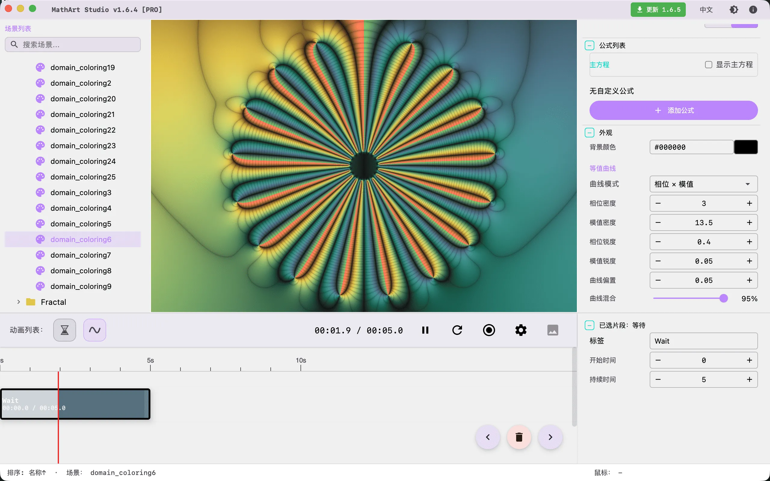
Interface Overview

All controls are located in the inspector panel on the right, divided into five main sections:

Geometry: Enter complex function formulas, adjust the viewport, and configure the iteration system
Settings: Switch between GPU/CPU rendering modes
Formulas: Display mathematical formulas and annotations
Appearance: Adjust background color, level curve parameters, and gradient palettes
Parameters: Define custom constants used in formulas

Note: Domain Coloring is a purely 2D scene and does not display the Camera panel.

Configuration Guide

1. Geometry (Geometry Settings)

Geometry Settings

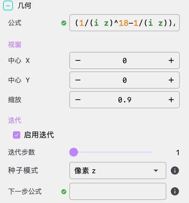
Formula Input

Formula input is the core of domain coloring. You can enter any complex function expression here, and the system will compile it into a GPU shader and render it in real time.

Supported Variables:

Variable	Meaning	Description
`z`	Pixel complex coordinate	Represents the position of the current pixel on the complex plane
`i`	Imaginary unit	i² = -1
`pi`	Circle constant π	≈ 3.14159
`e`	Euler's number e	≈ 2.71828
`c`	Complex constant	Defined by formula parameters a + bi
Custom parameters	e.g., `t`, `a`, `b`	Defined in the Parameters panel

Supported Operators:

Operator	Example	Description
`+`	`z + 1`	Complex addition
`-`	`z - i`	Complex subtraction
`*`	`z * i`	Complex multiplication (can be omitted: `2z` = `2*z`)
`/`	`1/z`	Complex division
`^`	`z^3`	Complex exponentiation

Supported Functions (25):

Category	Functions	Description
Trigonometric	`sin`, `cos`, `tan`	Complex trigonometric functions
Inverse trigonometric	`asin`, `acos`, `atan`, `acot`, `asec`, `acsc`	Complex inverse trigonometric functions
Hyperbolic	`sinh`, `cosh`, `tanh`	Complex hyperbolic functions
Inverse hyperbolic	`asinh`, `acosh`, `atanh`, `acoth`, `arsech`	Complex inverse hyperbolic functions
Exponential/Logarithmic	`exp`, `log`, `ln`	Complex exponential and logarithmic functions
Other	`sqrt`, `abs`, `arg`, `conj`, `pow`, `re`, `im`	Square root, absolute value, argument, conjugate, power, real part, imaginary part

Formula Examples:

Formula	Description
`z^3 - 1`	Cubic polynomial with three zeros
`sin(z)/cos(z)`	Tangent function tan(z)
`1/z`	Reciprocal function with a pole at z=0
`exp(1/z)`	Essential singularity with rich structure at z=0
`z^(a+3i)`	Complex power with parameter a controlling the exponent
`sin(z-i)/sin(z+i)`	Sine function with shifted poles
`sqrt(1-1/z^2+z^3)`	Composite function with square root

Tip: After modifying the formula, you need to click the "Apply" button for changes to take effect, because formula changes require shader recompilation.

Viewport Controls

Viewport controls determine the observation range of the complex plane:

Center X / Center Y: The center coordinates of the viewport on the complex plane
- Default: (0, 0)
- Step: 0.05, precision: 6 decimal places
- Tip: You can pan the viewport by dragging the canvas with the mouse
Scale: Zoom ratio
- Default: 2.5
- Range: 0.000001 ~ unlimited
- Smaller values show a larger area (zoom out); larger values show a smaller area (zoom in)
- Tip: You can zoom the viewport using the mouse scroll wheel

Operation tip: Mouse drag to pan + scroll wheel to zoom is the fastest way to explore, more intuitive than manually entering coordinates.

Iteration System

The iteration system is an advanced feature of domain coloring that extends single function evaluation to multiple iterations, enabling the generation of fractal patterns.

Iteration Settings

Enabling Iteration

Check the "Enable Iteration" toggle, and the system will perform multiple iteration calculations for each pixel instead of evaluating f(z) only once.

Iteration Steps

Steps: Number of iteration steps, range 1 - 64
More steps produce richer fractal detail but require more computation
Recommended starting point: 8-15 steps, then gradually increase to observe the effect

Seed Mode

The seed mode determines the initial value for iteration:

Mode	Initial Value	Typical Use	Example
PIXEL_Z	Pixel coordinate z	Mandelbrot set style	`w₀ = z`, `w_{k+1} = w_k² + c`
ZERO	0	Julia set style	`w₀ = 0`, `w_{k+1} = w_k² + z`
CONSTANT_C	Constant c	Newton fractal style	`w₀ = c`, `w_{k+1} = (w_k³-1)/(3w_k²) + c`

Understanding Seed Modes:
In PIXEL_Z mode, the iteration starting point for each pixel is its coordinate on the complex plane. This is the most intuitive mode, suitable for exploring the Mandelbrot set and its variants.
In ZERO mode, all pixels start iterating from 0, but z participates in the iteration formula as a parameter. This is suitable for generating Julia set patterns.
In CONSTANT_C mode, the iteration starting point is the constant c (defined by formula parameters), suitable for Newton's method for finding roots and similar applications.

Iteration Formula

The iteration formula uses the w variable for the current iteration value and z for the pixel coordinate:

Iteration Formula	Description
`w^2 + c`	Classic Mandelbrot/Julia iteration
`(w^3-1)/(3*w^2) + c`	Newton's method for roots of z³=1
`sin(w)cos(w)/(1+w)`	Trigonometric iteration
`sin(w + z^2)`	Composite iteration
`w`	Identity iteration (uses only the result of the initial formula)

Note: When the iteration formula is w, the system uses only the result of the initial formula f(z) as the iteration output. Combined with a higher number of iteration steps, this can produce a smooth accumulation effect.

2. Settings

Settings Panel

The settings panel for domain coloring is very simple, providing only the rendering mode switch:

GPU Mode (default): Uses OpenGL shaders for real-time rendering with the best performance
CPU Mode: Uses CPU per-pixel calculation as a fallback for the GPU mode

Recommendation: Always use GPU mode for the best performance. Switch to CPU mode only if GPU rendering has issues.

3. Formulas (Formula Display)

Display mathematical formulas and equation annotations in the scene.

Main Equation Display

Show Main Equation: Toggle the main equation display on/off
- When enabled, the system automatically displays the LaTeX formula in the scene based on the current formula
Position and Style:
- X / Y: Position coordinates of the formula in the scene
- Scale: Formula scaling ratio
- Color: Formula text color

Custom Formulas

You can add multiple custom formulas to the scene:

Click the "Add Formula" button to add a new formula
Each formula supports LaTeX content, position, scale, and color settings
Click the delete button in the top-right corner of a formula to remove it

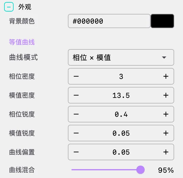
4. Appearance

Appearance Settings

Background Color

Background Color: Set the rendering background color
- Domain coloring typically uses dark backgrounds (such as #05070D or #000000) to highlight the function's color information

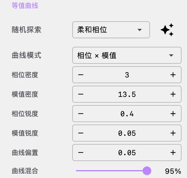
Level Curve

Level curves are the core visual control parameters of domain coloring, determining how the function's phase and modulus information is transformed into visible stripe patterns.

Curve Mode

Mode	Description	Use Case
PHASE	Display phase stripes only	Highlight argument variations; observe hue wheels at zeros and poles
MODULUS	Display modulus stripes only	Highlight modulus variations; observe constant-modulus curves
PHASE_MODULUS	Display both phase and modulus stripes	Most commonly used mode, combining both phase and modulus information
NONE	No level curves	Pure hue mapping, suitable for appreciating overall colors

Recommendation: Beginners should use PHASE_MODULUS mode, which provides the most information. Switch to PHASE mode when you want to focus on the hue structure of zeros and poles.

Phase Density

Range: 0.01 ~ unlimited
Default: 12.0
Step: 0.5
Effect: Controls the density of phase stripes. Higher values produce denser stripes with more frequent color changes
Suggestions:
- Low values (3-5): Wide stripes, suitable for observing large-scale hue variations
- Medium values (8-15): Standard density, balancing detail and readability
- High values (30+): Fine stripes, producing a contour-line-like effect

Modulus Density

Range: 0.01 ~ unlimited
Default: 8.0
Step: 0.5
Effect: Controls the density of modulus stripes. Higher values produce denser concentric ring patterns
Suggestions:
- Low values (5-8): Wide rings, suitable for observing overall modulus trends
- Medium values (10-18): Standard density
- High values (50+): Fine ring patterns, detailed display of modulus variations

Phase Sharpness

Range: 0.01 ~ unlimited
Default: 1.0
Step: 0.1
Effect: Controls the sharpness of phase stripes. Higher values produce sharper stripe boundaries; lower values produce softer stripes
Suggestions:
- 0.1-0.4: Soft gradients with smooth color transitions
- 0.5-1.0: Standard sharpness
- 1.0+: Sharp stripes with clearly distinguishable level curves

Modulus Sharpness

Range: 0.01 ~ unlimited
Default: 1.0
Step: 0.1
Effect: Controls the sharpness of modulus stripes, similar to phase sharpness

Curve Bias

Range: -1.0 ~ 1.0
Default: 0.15
Step: 0.05
Effect: Adjusts the overall brightness offset of level curves. Positive values brighten, negative values darken
Suggestions: Usually keep values close to 0; fine-tuning can improve the visual effect for specific functions

Curve Mix

Range: 0% ~ 100% (0.0 ~ 1.0)
Default: 100% (1.0)
Effect: Controls the blending ratio between level curves and pure hue mapping
- 0%: Pure hue mapping with no level curve effect
- 100%: Full level curve display
Suggestions: In most cases, keep 90%-100%; reducing the mix produces a softer visual effect

Gradient Palette

Domain coloring uses a 1D LUT (lookup table) texture for coloring, supporting three gradient modes:

Manual Mode:
- Manually add, delete, and adjust color nodes
- Supports drag-and-drop reordering of colors
- Random strategy selection (monochromatic, analogous, complementary, split-complementary)
Cosine Mode:
- Uses the IQ cosine palette formula: color(t) = a + b · cos(2π(c·t + d))
- Independently control offset, amplitude, frequency, and phase for R/G/B channels
- Supports one-click randomization and application
Curve Mode:
- Control R/G/B channels independently through editable Bézier curves
- Provides the most flexible color control
- Supports one-click randomization and application

Palette Selection Tips:
Classic domain coloring uses a rainbow palette (red → yellow → green → cyan → blue → magenta → red), corresponding to the hue wheel
Monochromatic palettes highlight level curve structure while de-emphasizing hue information
Contrasting palettes emphasize the positions of zeros and poles

5. Parameters

Define custom constants used in formulas. When a formula contains parameters (such as t, a, b, etc.), you need to define their values in this panel.

Add Parameter: Enter the parameter name and initial value at the bottom, then click the add button
Modify Parameter: Directly edit the parameter value
Delete Parameter: Click the delete button to the right of the parameter

Important: Parameters used in formulas must be defined in the Parameters panel first, otherwise formula validation will report an error. Parameter values can be dynamically changed in animations.

Animation and Timeline

Domain coloring supports rich animation effects that can be combined into continuous sequences through the timeline system.

Animation Types

Domain coloring supports two timeline animation types:

Wait: Maintain the current state for a specified duration
Animate: Execute a set of animation actions

Available Animation Methods

Method	Description	Parameters
`domainRotate`	Domain rotation animation	`rotation_speed`: rotation speed (float, default 0.2)
`paramStart`	Start parameter oscillation animation	Parameter configuration (see below)
`paramStop`	Stop parameter oscillation animation	None
`gradientStart`	Start gradient animation	Gradient configuration (see below)
`gradientStop`	Stop gradient animation	None

Parameter Oscillation Animation

Parameter oscillation animation makes parameters undergo periodic sinusoidal oscillation within a specified range — the most powerful animation feature of domain coloring.

How It Works

For each parameter, specify the step size, range (min, max), and edge easing
The parameter value oscillates sinusoidally within [min, max]: value = mid + amp × sin(phase)
The oscillation speed is controlled by the step size and step scale factor
Edge easing ensures the parameter decelerates near range boundaries, avoiding abrupt changes

Animatable Parameters

Parameter	Description	Default Animation Range
`scale`	Viewport scale	0.5 ~ 1.5
`phaseDensity`	Phase density	5.0 ~ 10.0
`modDensity`	Modulus density	5.0 ~ 10.0
`phaseSharpness`	Phase sharpness	0.001 ~ 2.0
`modSharpness`	Modulus sharpness	0.001 ~ 2.0
Custom parameters	e.g., `t`, `a`	-100 ~ 100

Edge Easing

Edge easing controls the speed variation of parameters at oscillation extremes, preventing hard bounces:

window: Easing window size (0-1); larger values produce wider easing intervals
floor: Minimum speed ratio during easing (0-1); 0 means complete stop
easing: Easing function type (e.g., SINE_OUT, QUAD_OUT, etc.)

Domain Rotation Animation

The domain rotation animation rotates the entire complex plane around the origin, producing a kaleidoscope-like visual effect:

Rotation speed is a floating-point number; positive values rotate clockwise, negative values counterclockwise
Typical values: 0.1 (slow rotation) ~ 0.5 (fast rotation)

Gradient Animation

Gradient animation shifts the palette cyclically, producing a color flow effect:

mode: Gradient mode, such as HUE_ROTATE (hue rotation)
speed: Animation speed
interpolation: Color interpolation mode (RGB, LINEAR, OKLAB, OKLCH)
affectInside / affectOutside: Whether to affect the inside/outside of level curves

Configuration Method

Define animation sequences through the timeline array in the JSON configuration file:

json

{
  "timeline": [
    { "type": "wait", "duration": 1 },
    {
      "type": "animate", "duration": 15, "easing": "SINE_IN_OUT",
      "actions": [
        { "method": "domainRotate", "args": [0.1] },
        {
          "method": "paramStart",
          "args": [{
            "targetDomain": "SURFACE",
            "parameters": {
              "t": { "step": 0.005, "min": 0.6, "max": 1.7,
                     "edgeEasing": { "window": 0.35, "floor": 0.4, "easing": "QUAD_OUT" } },
              "phaseDensity": { "step": 0.005, "min": 5, "max": 14 },
              "modDensity": { "step": 0.005, "min": 2, "max": 7 }
            }
          }]
        }
      ]
    },
    { "type": "wait", "duration": 30 }
  ]
}

Classic Domain Coloring Examples

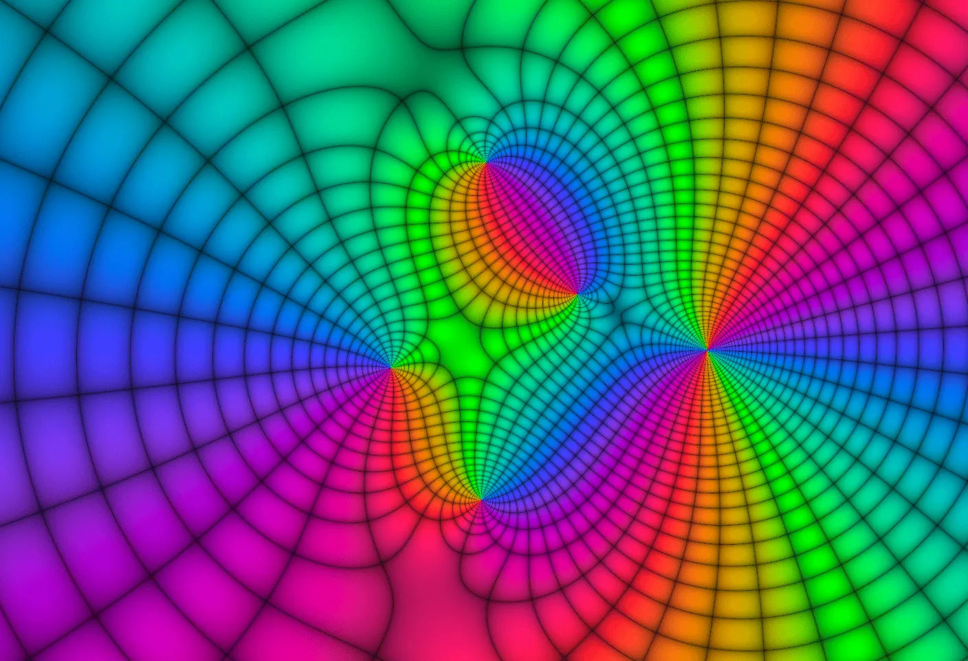
Example 1: Cubic Polynomial

The most classic domain coloring example, showing the hue wheel structure of three zeros.

Formula: z^3 - 1
Viewport: Center (0, 0), Scale 0.8
Level Curve: PHASE_MODULUS, Phase Density 20, Mod Density 17

Interpretation: The three zeros are located at 1, e^{2πi/3}, and e^{4πi/3}, appearing as three color convergence points in the image. The hue wheel completes one full cycle around each zero.

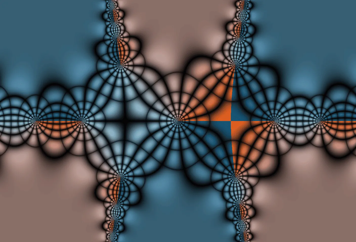
Example 2: Sine Function with Shifted Poles

Demonstrates the symmetric shifting of sine function poles.

Formula: sin(z-i)/sin(z+i)
Viewport: Center (0, 0), Scale 0.3
Level Curve: PHASE_MODULUS, Phase Density 4, Mod Density 16

Example 3: Parameterized Sine Function

Controls the sine function offset through parameter t, suitable for animation.

Formula: sin(z-1)/sin(z+t i)
Parameter: t = 0.95
Viewport: Center (0, 0), Scale 0.6
Level Curve: PHASE_MODULUS, Phase Density 4.5, Mod Density 13.5
Animation: Parameter t oscillates in range [2, -2]

Example 4: Complex Power

Complex power produces spiral domain coloring patterns with striking visual impact.

Formula: z^(a+3i)
Parameter: a = 1
Viewport: Center (0, 0), Scale 2.6
Level Curve: PHASE_MODULUS, Phase Density 4.5, Mod Density 13.5
Animation: Parameter a oscillates in range [1, 3]

Example 5: Newton Fractal

Uses Newton's iteration method to find the roots of z³ = 1, generating the classic Newton fractal pattern.

Formula: z (identity mapping)
Iteration: Enabled, Seed Mode CONSTANT_C, Steps 8
Iteration Formula: (w^3-1)/(3*w^2) + c
Viewport: Center (0, 0), Scale 0.5
Level Curve: PHASE_MODULUS, Phase Density 13, Mod Density 7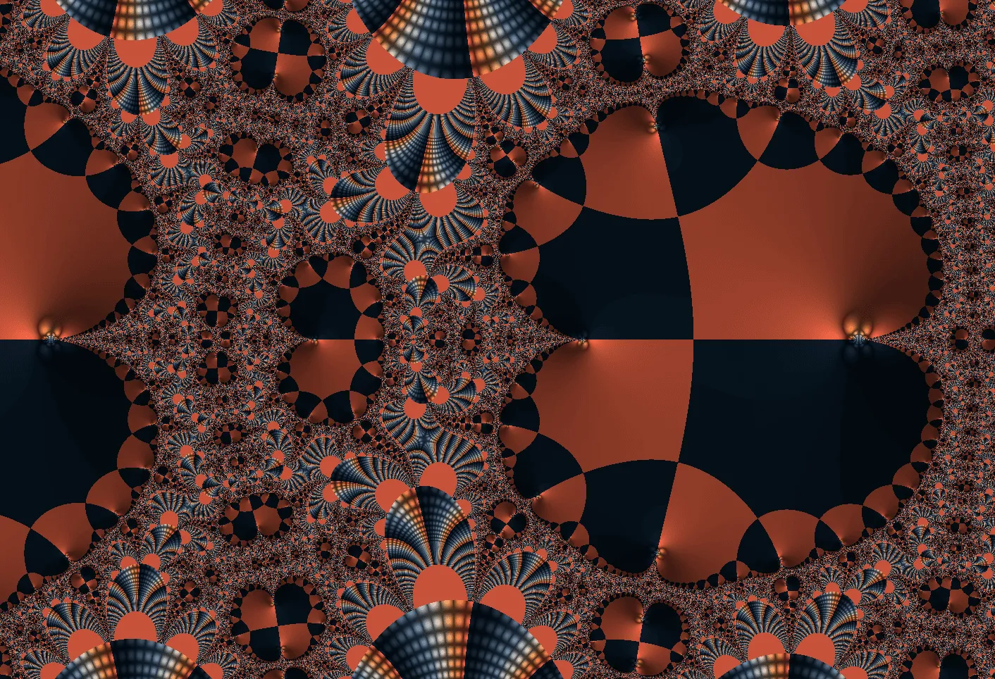

Newton Fractal

Interpretation: Newton's method divides the complex plane into three basins (corresponding to the three roots), each represented by a different color. The boundaries between basins exhibit fractal structure — no matter how much you zoom in, the boundaries maintain complex detail.

Example 6: Trigonometric Iteration

Fractal patterns generated using trigonometric function iteration.

Formula: z (identity mapping)
Iteration: Enabled, Seed Mode PIXEL_Z, Steps 45
Iteration Formula: sin(w)cos(w)/(1+w)
Escape Radius: 64
Viewport: Center (-0.5, 0), Scale 0.5
Level Curve: PHASE_MODULUS, Phase Density 10, Mod Density 6

Example 7: ZERO Seed Iteration

Iteration starting from zero, generating Julia set style patterns.

Formula: z (identity mapping)
Iteration: Enabled, Seed Mode ZERO, Steps 27
Iteration Formula: sin(w + z^2)
Escape Radius: 1024
Viewport: Center (0, 0), Scale 1.2
Level Curve: PHASE_MODULUS, Phase Density 9, Mod Density 5

Example 8: Rational Function

Domain coloring of a rational function shows the interwoven structure of zeros and poles.

Formula: ((z^2 - 1)(z - 2 - i)^2) / (z^2 + 2 + 2i)
Viewport: Center (0, 0), Scale 0.3
Level Curve: PHASE_MODULUS, Phase Density 5, Mod Density 18

More Showcase

Domain Coloring Example 1 Domain Coloring Example 2

Technical Details

GPU Rendering Pipeline

Domain coloring uses a single-pass GPU rendering pipeline:

Vertex Shader: Performs MVP transformation and passes UV coordinates
Fragment Shader (core rendering logic):
- UV → complex plane coordinate mapping (with aspect ratio correction and rotation)
- Formula evaluation (with iteration)
- Overflow protection (marks values where |f(z)|² > 10²⁴)
- Compute modulus and argument
- Generate phase stripes and modulus stripes (based on cosine functions)
- Palette sampling + level curve blending + bias

Dynamic Shader Compilation

The most sophisticated technical implementation of domain coloring is dynamic shader compilation:

Formula Parsing: ComplexExpressionParser parses the string formula (e.g., z^3 - tan(t*z)) into an Abstract Syntax Tree (AST)
GLSL Code Generation: The AST is converted to a GLSL expression (e.g., c_sub(c_pow_int(z, 3), c_mul(c_tan(c_mul(t, z)), vec2(1.0, 0.0))))
Shader Injection: Dynamic formula macros and parameter declarations are inserted into the standard shader source code
Caching Mechanism: Recompilation is avoided by comparing with the previously compiled GLSL code

Complex Number Library

The shader includes a complete GLSL complex number library with 25 complex functions. The Java and GLSL implementations are fully consistent, ensuring that CPU and GPU paths produce identical results.

Creative Tips

Formula Exploration

Start Simple: Try basic functions like z^2, 1/z, sin(z) first to understand the visual language of domain coloring
Combine Functions: Combine basic functions, e.g., sin(z)/cos(z) = tan(z), and observe the relationship between zeros and poles
Introduce Parameters: Add parameter t to formulas, e.g., z^3 - tan(t*z), then animate the parameter
Try Iteration: Enable the iteration system and use iteration formulas like w^2 + c to generate fractals

Visual Tuning

Level Curve Adjustment:
- Start with PHASE_MODULUS mode for complete information
- Adjust phase density and modulus density for appropriate stripe spacing
- Adjust sharpness for clear but not harsh stripe boundaries
- Fine-tune mix and bias for the best visual effect
Palette Selection:
- Rainbow palette: The most classic domain coloring palette, corresponding to the hue wheel
- Warm-cool palette: Highlights the contrast between zeros (warm colors) and poles (cool colors)
- Monochromatic palette: Highlights level curve structure while de-emphasizing hue information
Viewport Control:
- Use mouse drag and scroll wheel for quick navigation to areas of interest
- Zoom in near zeros or poles to observe fine fractal structures

Animation Design

Parameter Oscillation:
- Set oscillation animation for parameter t in the formula to observe continuous morphological changes
- Simultaneously oscillate phaseDensity and modDensity for a "breathing" effect
- Use edge easing to avoid abrupt changes at parameter extremes
Domain Rotation:
- Combine domain rotation with parameter oscillation for a rotating kaleidoscope effect
- Recommended rotation speed: 0.05-0.2; faster speeds can be disorienting
Gradient Animation:
- Use HUE_ROTATE mode for cyclic palette flow
- OKLAB interpolation mode produces more natural color transitions than RGB mode

FAQ

Image is Completely Black or White

Problem: The rendering result is entirely black or entirely white

Cause: The function values are too large or too small in certain regions, compressing the color information

Solution:

Adjust Scale to change the observation range
Adjust level curve parameters: increase phaseDensity and modDensity
Check if the function is defined in the current viewport range (e.g., 1/z is undefined at z=0)

Formula Compilation Failure

Problem: Compilation error after entering a formula

Cause: Incorrect formula syntax or use of unsupported functions

Solution:

Ensure you use supported function names (case-sensitive)
Ensure all parameters used are defined in the Parameters panel
Check that parentheses are properly matched
Use * for multiplication (2z can be omitted, but z(z+1) is recommended to be written as z*(z+1))

Unsatisfactory Iteration Results

Problem: The image effect after enabling iteration is not as expected

Cause: Improper iteration parameter configuration

Solution:

Try different seed modes (PIXEL_Z / ZERO / CONSTANT_C)
Adjust iteration steps (start from 8-15 steps)
Check if the iteration formula is correct
Adjust the escape radius (default 1,000,000; some functions may need smaller values)

Shader Compilation Stuttering

Problem: Brief stuttering after modifying the formula

Cause: Formula changes require GPU shader recompilation

Solution:

This is normal behavior; compilation typically completes within 0.5 seconds
Only formula and iteration formula changes require recompilation; other parameter modifications update in real time

Advanced Topics

Understanding Local Behavior of Complex Functions

Domain coloring is a powerful tool for understanding the local behavior of complex functions:

Zeros: Near a zero, f(z) ≈ a·(z-z₀)ⁿ, the hue wheel cycles n times
Poles: Near a pole, f(z) ≈ a/(z-z₀)ⁿ, the hue wheel cycles in reverse n times
Essential singularities: Near an essential singularity (e.g., exp(1/z) at z=0), color changes are extremely dramatic, showing "infinite oscillation"

The Relationship Between Mandelbrot and Julia Sets

Through the domain coloring iteration system, you can explore both the Mandelbrot set and Julia sets:

Mandelbrot Set: Use PIXEL_Z seed mode with iteration formula w^2 + c, where c is a constant. Each pixel z serves as the initial value, and c as a parameter
Julia Set: Use ZERO seed mode with iteration formula w^2 + z, where z is the pixel coordinate. All pixels start iterating from 0, with z as a parameter

The relationship between the two: each point c in the Mandelbrot set corresponds to a Julia set. Points c inside the Mandelbrot set produce connected Julia sets, while points outside produce disconnected Julia sets (Fatou dust).

Mathematical Principles of Newton Fractals

When using Newton's method to find roots of f(z) = 0, the iteration formula is:

For f(z) = z³ - 1, the iteration formula becomes:

The fascination of Newton fractals lies in this: although the three roots are simple points, the boundaries of their basins of attraction are infinitely complex fractals — another example of the coexistence of chaos and order.

References

Mathematical Theory

Tristan Needham - Visual Complex Analysis (1997) - Classic textbook on visual complex analysis
Elias Wegert - Visual Complex Functions: An Introduction with Phase Portraits (2012) - Systematic treatment of domain coloring methods
Frank Farris - "Visualizing complex-valued functions in the plane" (1997) - Paper popularizing the domain coloring method

Online Resources

Wikipedia: Domain Coloring
Wikipedia: Complex Analysis
Complex Analysis - MIT OpenCourseWare - MIT complex analysis open course

Complex Explorer - Online domain coloring tool
Wolfram Alpha - Supports complex function visualization

Domain Coloring ​

Introduction ​

Mathematical Background ​

What is Domain Coloring? ​

Coloring Principles of Domain Coloring ​

Key Features in Domain Coloring Images ​

Historical Background ​

Interface Overview ​

Configuration Guide ​

1. Geometry (Geometry Settings) ​

Formula Input ​

Viewport Controls ​

Iteration System ​

Enabling Iteration ​

Iteration Steps ​

Seed Mode ​

Iteration Formula ​

2. Settings ​

3. Formulas (Formula Display) ​

Main Equation Display ​

Custom Formulas ​

4. Appearance ​

Background Color ​

Level Curve ​

Curve Mode ​

Phase Density ​

Modulus Density ​

Phase Sharpness ​

Modulus Sharpness ​

Curve Bias ​

Curve Mix ​

Gradient Palette ​

5. Parameters ​

Animation and Timeline ​

Animation Types ​

Available Animation Methods ​

Parameter Oscillation Animation ​

How It Works ​

Animatable Parameters ​

Edge Easing ​

Domain Rotation Animation ​

Gradient Animation ​

Configuration Method ​

Classic Domain Coloring Examples ​

Example 1: Cubic Polynomial ​

Example 2: Sine Function with Shifted Poles ​

Example 3: Parameterized Sine Function ​

Example 4: Complex Power ​

Example 5: Newton Fractal ​

Example 6: Trigonometric Iteration ​

Example 7: ZERO Seed Iteration ​

Example 8: Rational Function ​

More Showcase ​

Technical Details ​

GPU Rendering Pipeline ​

Dynamic Shader Compilation ​

Complex Number Library ​

Creative Tips ​

Formula Exploration ​

Visual Tuning ​

Animation Design ​

FAQ ​

Image is Completely Black or White ​

Formula Compilation Failure ​

Unsatisfactory Iteration Results ​

Shader Compilation Stuttering ​

Advanced Topics ​

Understanding Local Behavior of Complex Functions ​

The Relationship Between Mandelbrot and Julia Sets ​

Mathematical Principles of Newton Fractals ​

References ​

Mathematical Theory ​

Online Resources ​

Related Software ​

Domain Coloring

Introduction

Mathematical Background

What is Domain Coloring?

Coloring Principles of Domain Coloring

Key Features in Domain Coloring Images

Historical Background

Interface Overview

Configuration Guide

1. Geometry (Geometry Settings)

Formula Input

Viewport Controls

Iteration System

Enabling Iteration

Iteration Steps

Seed Mode

Iteration Formula

2. Settings

3. Formulas (Formula Display)

Main Equation Display

Custom Formulas

4. Appearance

Background Color

Level Curve

Curve Mode

Phase Density

Modulus Density

Phase Sharpness

Modulus Sharpness

Curve Bias

Curve Mix

Gradient Palette

5. Parameters

Animation and Timeline

Animation Types

Available Animation Methods

Parameter Oscillation Animation

How It Works

Animatable Parameters

Edge Easing

Domain Rotation Animation

Gradient Animation

Configuration Method

Classic Domain Coloring Examples

Example 1: Cubic Polynomial

Example 2: Sine Function with Shifted Poles

Example 3: Parameterized Sine Function

Example 4: Complex Power

Example 5: Newton Fractal

Example 6: Trigonometric Iteration

Example 7: ZERO Seed Iteration

Example 8: Rational Function

More Showcase

Technical Details

GPU Rendering Pipeline

Dynamic Shader Compilation

Complex Number Library

Creative Tips

Formula Exploration

Visual Tuning

Animation Design

FAQ

Image is Completely Black or White

Formula Compilation Failure

Unsatisfactory Iteration Results

Shader Compilation Stuttering

Advanced Topics

Understanding Local Behavior of Complex Functions

The Relationship Between Mandelbrot and Julia Sets

Mathematical Principles of Newton Fractals

References

Mathematical Theory

Online Resources

Related Software