Map Attractor

Introduction

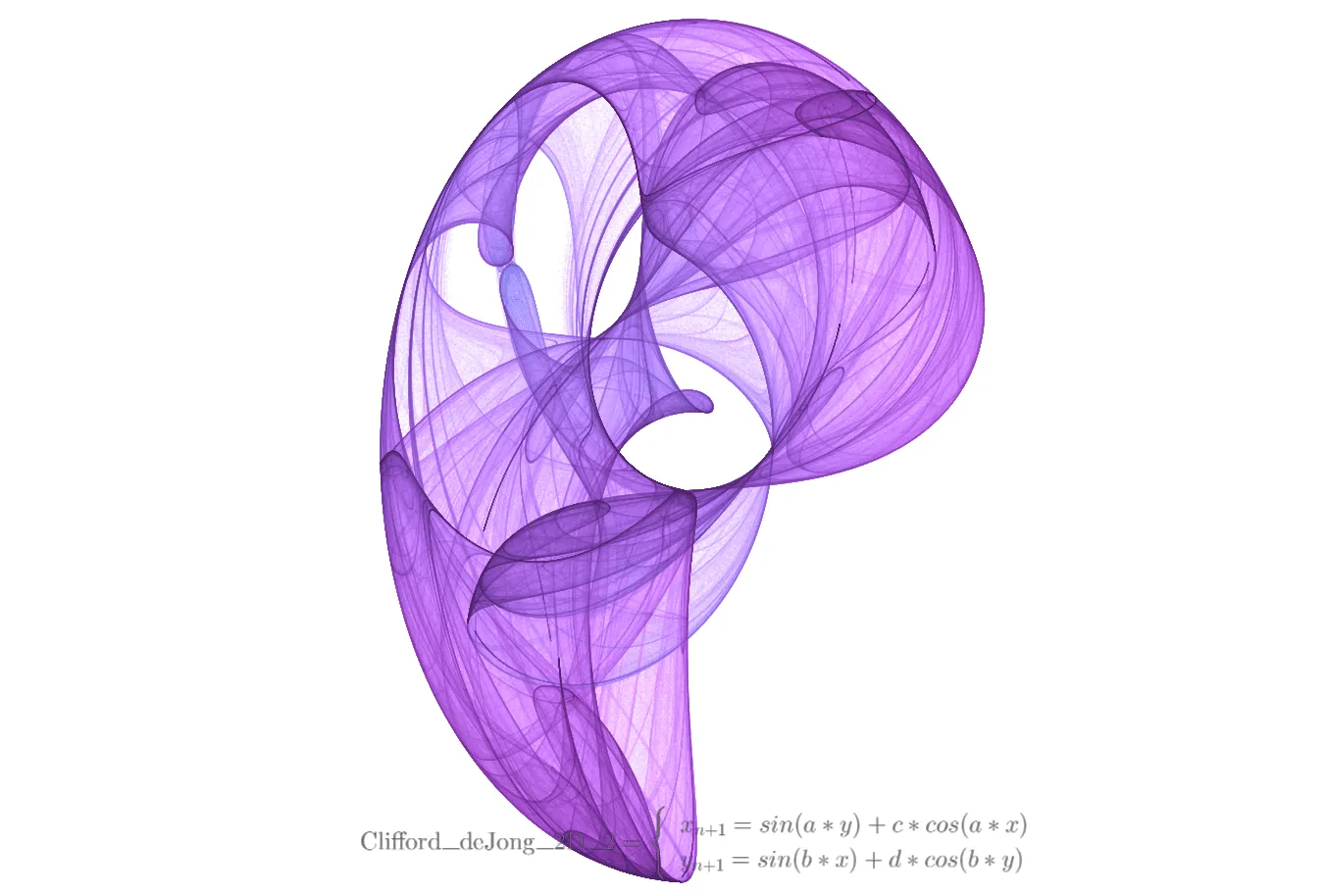
Map attractors transform iterated maps into high-density visual art. By parallel-iterating hundreds of thousands of particles on the GPU and employing density accumulation and tone mapping techniques, you can create attractor images with extremely high visual fidelity — this is the standard rendering approach for classic map attractors such as the Clifford attractor and the Peter de Jong attractor.

Key Capabilities:

• High-Performance GPU Rendering: Pure GPU pipeline supporting parallel iteration and density accumulation for hundreds of thousands of particles
• Iterated Map System: Supports 2D and 3D map equations, with y_next able to reference the computed result of x_next
• Professional Tone Mapping: Built-in complete tone control chain including brightness, contrast, gamma, dynamic range, saturation, and more
• Step Metric Coloring: Coloring based on per-step particle displacement, revealing the attractor's motion characteristics
• Full Animation Support: Integrated parameter oscillation animation system supporting smooth periodic parameter changes

---

Mathematical Background

What is a Map Attractor?

A map attractor (also known as an iterated map attractor) is a type of discrete dynamical system. Unlike strange attractors (continuous systems defined by differential equations), map attractors compute the next state directly through iterative functions:

Key Differences from Strange Attractors:

Feature	Strange Attractor	Map Attractor
System Type	Continuous (differential equations)	Discrete (iterated map)
Iteration Method	Numerical integration (Euler, etc.)	Direct function computation
Rendering Method	Particle trails	Density accumulation
Classic Examples	Lorenz, Rossler	Clifford, Peter de Jong

Cascaded Computation of Map Equations

An important feature of map attractors is the cascaded dependency between equations:

1. x_next depends only on the current state (x, y, z) and custom parameters
2. y_next can reference x_next (also written as nx), meaning y's computation can utilize x's new value
3. z_next (3D mode) can reference x_next/nx and y_next/ny

This cascaded design enables map attractors to express richer dynamical behaviors.

Classic Examples

Clifford Attractor (2D):

x_next = sin(a * y) + c * cos(a * x)
y_next = sin(b * x) + d * cos(b * y)
Parameters: a = -1.7, b = 1.8, c = 1.6, d = 0.9

Peter de Jong Attractor (2D):

x_next = sin(a * y) - cos(b * x)
y_next = sin(c * x) - cos(d * y)
Parameters: a = -2.24, b = 0.43, c = -0.65, d = -2.43

3D Map Attractor:

x_next = sin(a * y) + c * cos(a * x)
y_next = sin(b * x) + d * cos(b * y)
z_next = sin(e * x) + f * cos(e * z)

---

Interface Overview

All controls are located in the inspector panel on the right, divided into six main sections:

1. Geometry: Define map equations and spatial transforms
2. Parameters: Define custom constants used in equations
3. Simulation: Configure iteration properties, tone mapping, and coloring parameters
4. Camera: Control viewing angles
5. Formulas: Display mathematical formulas and annotations
6. Appearance: Adjust background color and other rendering settings

---

Configuration Guide

1. Geometry (Map Equations)

This section defines the system's iterative map functions.

Map Equations

• x_next: Map equation for computing the next x value

  • Supported Variables: x, y, z (current state coordinates) and custom parameters
  • Example: sin(a * y) + c * cos(a * x)

• y_next: Map equation for computing the next y value

  • Supported Variables: x, y, z, x_next (or nx) and custom parameters
  • Cascade Reference: Can reference the computed result of x_next
  • Example: sin(b * x) + d * cos(b * y)

• z_next (3D mode only): Map equation for computing the next z value

  • Supported Variables: x, y, z, x_next/nx, y_next/ny and custom parameters
  • Cascade Reference: Can reference computed results of x_next and y_next
  • Example: sin(e * x) + f * cos(e * z)

• Supported Functions: sin, cos, tan, asin, acos, atan, sinh, cosh, tanh, sqrt, abs, log, ln, log10, exp, floor, ceil, round, sign, pow, min, max, atan2, etc.

Spatial Transform

• Scale X/Y/Z: Adjust the size of the attractor in the scene
• Offset X/Y/Z: Adjust the position of the attractor in the scene
• Tip: Different map equations produce vastly different numerical ranges. Use Scale to fit the attractor within appropriate camera view

---

2. Parameters (Custom Constants)

It is recommended not to hardcode numbers in equations but define named parameters here.

• Add Parameter: Create variables like a, b, c, d
• Usage: Use these variable names directly in the Geometry panel equations
• Live Tuning: Modifying these values during playback can dynamically evolve the attractor's shape
• Advantages:
  • Convenient for adjustment and experimentation
  • Supports parameter oscillation animation
  • Improves configuration readability and maintainability

---

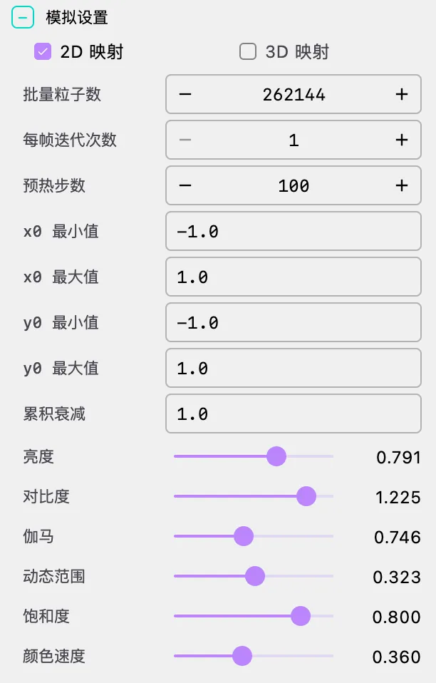
3. Simulation (Simulation Settings)

Controls the system's iteration behavior and visual presentation. Map attractors use a pure GPU rendering pipeline with no CPU/GPU mode switching.

Dimension Selection

• 2D / 3D: Select the dimension of the map attractor
  • 2D Mode: Only x_next and y_next equations are used; z_next is automatically set to 0
  • 3D Mode: All three equations are used, supporting attractor structures in three-dimensional space
  • Note: When switching dimensions, the z_next equation will be reset. Switching from 3D to 2D clears z_next; switching from 2D to 3D sets z_next to z by default

Iteration Settings

• Batch Size: Number of particles iterated in parallel

  • Purpose: Determines the total number of particles participating in computation per frame
  • Default: 262,144 (approximately 260K)
  • Recommendations:
    • Simple maps (e.g., Clifford): 100,000 - 500,000
    • Complex maps: 50,000 - 200,000
  • Note: Excessively large Batch Size consumes significant GPU video memory and may cause rendering stuttering

• Iterations Per Frame: Number of map iterations executed per render frame

  • Range: 1 - 16
  • Purpose: Controls the speed of attractor density accumulation
  • Recommendation: Typically set to 1; increasing this value fills the attractor more quickly

• Burn-In Steps: Number of iterations to pre-compute before drawing the first frame

  • Purpose: Guides particles from initial positions onto attractor orbits
  • Recommendation: At least 50 steps to avoid visual abruptness from initial random distribution

Initial Range

• X₀ Min / X₀ Max: Range for initial particle x coordinates
• Y₀ Min / Y₀ Max: Range for initial particle y coordinates
  • Default: [-1.0, 1.0]
  • Tip: Initial range selection affects burn-in effectiveness. For maps where the attractor occupies a larger range, you may need to expand the initial range

Density and Tone Mapping

Map attractors use a density accumulation + tone mapping rendering pipeline, which is the core technique for generating high-quality map attractor images.

• Accumulation Decay: Controls the retention of historical density data

  • Range: 0.0 - 1.0
  • Default: 1.0 (full retention)
  • Purpose: At 1.0, density fully accumulates; lowering this value causes older density to gradually decay, producing a "fade-out" effect
  • Recommendation: Keep at 1.0 for complete attractor images; lower to 0.9-0.99 to observe transition effects during parameter changes

• Brightness: Overall brightness offset

  • Range: -0.5 - 1.5
  • Default: 0.3
  • Purpose: Adjusts the overall brightness of accumulated density

• Contrast: Contrast of the density distribution

  • Range: 0.1 - 2.0
  • Default: 1.0
  • Purpose: Enhances or reduces the light-dark contrast of the density distribution

• Gamma: Non-linear brightness mapping

  • Range: 0.1 - 10.0
  • Default: 2.2
  • Purpose: Controls mid-tone brightness. Larger values reveal more shadow detail; smaller values emphasize highlights
  • Recommendation: 2.2 is the standard sRGB gamma value, suitable for most scenarios

• Dynamic Range: Dynamic range of density mapping

  • Range: 0.1 - 1.0
  • Default: 0.2
  • Purpose: Controls the density-to-luminance mapping range. Smaller values make the attractor brighter; larger values preserve more shadow detail

• Saturation: Color saturation

  • Range: 0.0 - 1.0
  • Default: 0.8
  • Purpose: 0.0 is grayscale, 1.0 is fully saturated

Step Metric Coloring

Step metric is a coloring method unique to map attractors, assigning colors based on each particle's per-step displacement.

• Step Metric Min / Max: Normalization range for step metric

  • Purpose: Maps each particle's per-step displacement to the [Min, Max] range for coloring
  • Recommendations:
    • Min is typically set to 0.0
    • Max should be adjusted based on the attractor's characteristics, typical values 1.0 - 3.0
  • Note: Max must be greater than Min; the system automatically ensures Max ≥ Min + 0.001

• Color Speed: Color cycling speed

  • Range: 0.1 - 2.0
  • Default: 0.22
  • Purpose: Controls the frequency of color cycling through the palette

• Color Phase: Color cycling starting phase

  • Range: 0.0 - 360.0
  • Default: 180.0
  • Purpose: Offsets the starting position of color mapping, equivalent to rotating the palette

• Invert: Invert brightness

  • Purpose: Swaps light and dark colors, producing a negative effect
  • Use Cases: Light attractor on dark background ↔ Dark attractor on light background

---

4. Camera (Camera Control)

Adjust viewing angles and camera parameters.

Camera Angles

• Phi (Pitch Angle): Vertical angle of the camera

  • Range: 0 to π (0 to 180 degrees)
  • Default: π/2 (90 degrees, horizontal view)

• Theta (Yaw Angle): Horizontal angle of the camera

  • Range: 0 to 2π (0 to 360 degrees)
  • Default: 0

• Gamma (Roll Angle): Rotation angle of the camera

  • Range: 0 to 2π (0 to 360 degrees)
  • Default: 0

Usage Tips

• 2D Attractors: Typically use top-down view (Phi = 0 or π) or horizontal view (Phi = π/2)
• 3D Attractors: Observe the 3D structure from different angles by adjusting Phi and Theta
• Animation Effects: Create camera rotation animations with the timeline system

---

5. Formulas (Formula Display)

Display mathematical formulas and equations in the scene.

Main Equation Display

• Show Main Equation: Toggle main equation display on/off

  • Purpose: Display the iterative equations of the current map attractor in the scene
  • Auto-generation: The system automatically generates LaTeX formulas based on current equations and parameters

• Main Equation Position:

  • X: Horizontal position coordinate
  • Y: Vertical position coordinate
  • Scale: Formula scaling ratio
  • Color: Formula color

Custom Formulas

Add multiple custom formulas to the scene:

• Add Formula: Click "Add Formula" button to add a new formula
• Formula Content:
  • LaTeX: Mathematical formula in LaTeX format
  • X: Horizontal position coordinate
  • Y: Vertical position coordinate
  • Scale: Formula scaling ratio
  • Color: Formula color
• Delete Formula: Click the delete button in the top-right corner of the formula to remove it

---

Animation and Timeline

Parameter Oscillation Animation

Map attractors support Parameter Oscillation Animation, a unique animation method that allows parameters to undergo periodic sinusoidal oscillation within a specified range.

How It Works

Parameter oscillation animation is implemented through MapAttractorParameterAnimator:

1. For each parameter, specify the oscillation step, range (min, max), and edge easing
2. The parameter value oscillates sinusoidally within [min, max]: value = mid + amp * sin(phase)
3. Oscillation speed is jointly controlled by the step and step scale factor
4. Edge easing ensures the parameter decelerates near range boundaries, avoiding abrupt changes

Animation Types

• StartMapAttractorParamAnimation: Start parameter oscillation animation

  • Can start for a single parameter or for all parameters simultaneously
  • Step scale gradually increases from 0 to 1 on start, achieving a smooth transition
  • Configuration parameters:
    • paramName: Parameter name (null affects all parameters)
    • step: Oscillation step (positive for forward, negative for reverse oscillation)
    • min: Oscillation range lower bound
    • max: Oscillation range upper bound
    • duration: Start transition duration
    • edgeEasing: Edge easing configuration

• StopMapAttractorParamAnimation: Stop parameter oscillation animation

  • Step scale gradually decreases from current value to 0, achieving a smooth stop

Animatable Special Parameters

In addition to custom parameters, the following system parameters also support animation:

• colorSpeed: Color cycling speed
• colorPhase: Color phase offset

Camera Animation

Map attractors also support standard camera animations:

• Rotation: Rotate camera around the attractor
• Alignment: Align camera to specific angles
• Zoom: Adjust camera distance

Configuration Method

Define animation sequences through the timeline array in JSON configuration:

{
  "timeline": [
    {
      "type": "animate",
      "duration": 15.0,
      "easing": "SINE_IN_OUT",
      "actions": [
        {"method": "rotateTheta", "args": [6.283]}
      ]
    },
    {
      "type": "hold",
      "duration": 2.0
    }
  ]
}

---

Performance & Best Practices

Recommended Configurations

Goal	Batch Size	Iterations/Frame	Burn-In Steps	Gamma	Dynamic Range
High Quality Image	500,000+	1	200+	2.2	0.15-0.25
Real-time Interaction	100,000-200,000	1-2	50-100	2.2	0.2-0.3
Parameter Exploration	50,000-100,000	1	50	2.2	0.2

Performance Optimization Tips

1. Batch Size Adjustment:

   • Reducing Batch Size is the most direct performance optimization
   • Complex equations (with multiple trigonometric functions) should use smaller Batch Size

2. Tone Mapping Tuning:

   • Increasing Dynamic Range makes more detail visible, but may require adjusting Brightness accordingly
   • Gamma significantly affects visual results; 2.2 is a good starting point

3. Burn-In Optimization:

   • Appropriate burn-in steps avoid visual noise in initial frames
   • Excessive burn-in steps increase scene loading time

4. Rebuilding on Parameter Changes:

   • Modifying equations or parameters automatically triggers accumulation buffer rebuild (Replay)
   • The rebuild process progressively refills density, avoiding sudden visual jumps
   • Frequent parameter changes may cause repeated rebuilds; consider adjusting parameters while paused

---

Troubleshooting

Completely Black or White Image

Problem: Rendered result is entirely black or entirely white

Cause: Tone mapping parameters don't match the current attractor's density distribution

Solutions:

• Adjust Brightness (increase when black, decrease when white)
• Adjust Dynamic Range (decrease when black, increase when white)
• Adjust Gamma (increase gamma when black)
• Check if Batch Size is large enough to produce visible density

Incomplete Attractor Shape

Problem: Attractor shows only partial structure

Cause: Insufficient burn-in steps or initial range too small

Solutions:

• Increase Burn-In Steps (e.g., from 50 to 200)
• Expand initial range (X₀ and Y₀ Min/Max)
• Increase Iterations Per Frame to accelerate density accumulation

Particle Divergence

Problem: Image shows uniform noise or is completely blurry

Cause: Map equation does not produce a bounded attractor

Solutions:

• Check if the equation is correct — not all maps produce attractors
• Try classic parameter combinations (e.g., Clifford attractor parameters)
• Certain parameter combinations cause iterative divergence; this is a mathematical property of the map itself, not a software error

Unsatisfactory Colors

Problem: Colors appear monotonous or lack depth

Cause: Step metric range or color parameter settings are inappropriate

Solutions:

• Adjust Step Metric Min/Max to match the attractor's actual step size distribution
• Adjust Color Speed to change color cycling frequency
• Adjust Color Phase to offset the color starting position
• Adjust Saturation to increase or decrease color saturation

Flickering When Modifying Parameters

Problem: Screen flickers or jumps when modifying parameters

Cause: Parameter changes trigger accumulation buffer rebuild

Solutions:

• This is normal behavior — the system needs to rebuild density accumulation to reflect new parameters
• The rebuild process typically completes within 0.5 seconds
• If flickering is too frequent, consider adjusting parameters while paused

---

Classic Map Attractor Examples

Clifford Attractor

{
  "type": "MAP_ATTRACTOR",
  "dimension": 2,
  "equations": {
    "x_next": "sin(a * y) + c * cos(a * x)",
    "y_next": "sin(b * x) + d * cos(b * y)"
  },
  "parameters": {
    "a": -1.7,
    "b": 1.8,
    "c": 1.6,
    "d": 0.9
  }
}

Peter de Jong Attractor

{
  "type": "MAP_ATTRACTOR",
  "dimension": 2,
  "equations": {
    "x_next": "sin(a * y) - cos(b * x)",
    "y_next": "sin(c * x) - cos(d * y)"
  },
  "parameters": {
    "a": -2.24,
    "b": 0.43,
    "c": -0.65,
    "d": -2.43
  }
}

Cascaded Map Attractor (y_next references x_next)

{
  "type": "MAP_ATTRACTOR",
  "dimension": 2,
  "equations": {
    "x_next": "sin(a * y) + c * cos(a * x)",
    "y_next": "sin(b * nx) + d * cos(b * y)"
  },
  "parameters": {
    "a": -1.4,
    "b": 1.6,
    "c": 1.0,
    "d": 0.7
  }
}

3D Map Attractor

{
  "type": "MAP_ATTRACTOR",
  "dimension": 3,
  "equations": {
    "x_next": "sin(a * y) + c * cos(a * x)",
    "y_next": "sin(b * x) + d * cos(b * y)",
    "z_next": "sin(e * x) + f * cos(e * z)"
  },
  "parameters": {
    "a": -1.7,
    "b": 1.8,
    "c": 1.6,
    "d": 0.9,
    "e": -0.5,
    "f": 1.2
  }
}

---

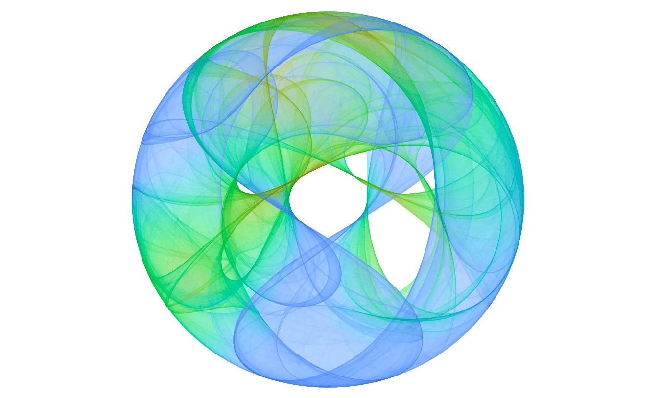
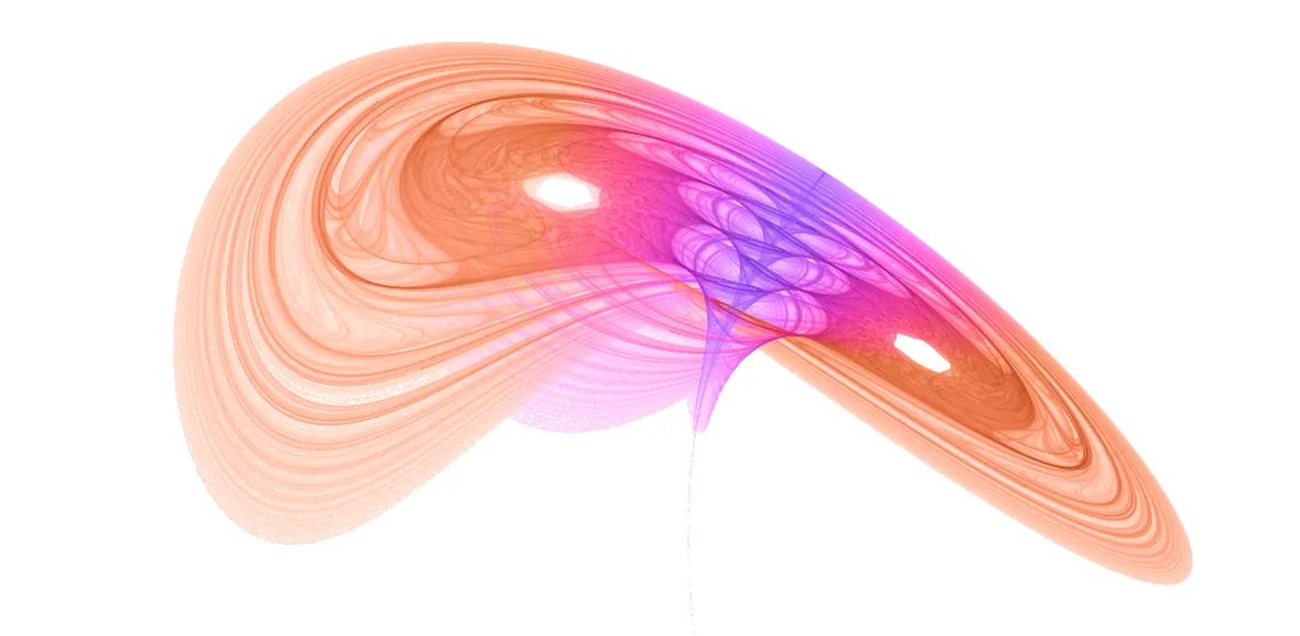
More Visual Examples

---

Technical Details

GPU Rendering Pipeline

Map attractors use a three-pass GPU rendering pipeline:

1. Update Pass:

   • Reads current particle state texture (position + step metric)
   • Executes map equations to compute the next state
   • Uses Ping-Pong double buffering for alternating state read/write

2. Accumulate Pass:

   • Projects particle positions to screen space
   • Uses additive blending to accumulate particle density into a floating-point texture
   • Supports accumulation decay for dynamic effects

3. Present Pass:

   • Applies tone mapping chain to accumulated density: brightness → contrast → gamma → dynamic range → saturation → invert
   • Auto-scaling factor computed from accumulated sample count and viewport size, ensuring visual consistency across resolutions

Shader Compilation

Map equations are compiled to GLSL shader code at runtime:

• MapAttractorExpressionCompiler converts user-input mathematical expressions to GLSL
• Custom parameters are passed through uniform variables; modifying parameter values does not require shader recompilation
• Shader recompilation is only needed when a new parameter symbol is added

Replay Mechanism

When parameters or camera change, the system triggers a Replay rebuild:

• Resets particle state to initial positions
• Re-executes burn-in iterations
• Progressively re-accumulates density (completes within approximately 0.5 seconds)
• Ensures smooth visual transitions, avoiding sudden jumps

---

Creative Techniques

Parameter Exploration

1. Start from Classics: First use known classic parameter values for Clifford or Peter de Jong
2. Small Range Adjustments: Adjust parameters in small ranges around classic values and observe shape changes
3. Cascade Experiments: Try referencing x_next in y_next to create more complex dynamics
4. Record Discoveries: Save interesting parameter combinations

Visual Tuning

1. Tone Mapping:

   • First adjust Dynamic Range to make the overall attractor visible
   • Then adjust Gamma to reveal mid-tone details
   • Finally fine-tune Brightness and Contrast

2. Color Schemes:

   • Adjust Color Speed and Color Phase to create rich color variations
   • Lowering Saturation can produce more elegant visual effects
   • Use Invert to switch between light and dark styles

3. Step Metric:

   • Step Metric Max determines the sensitivity range of coloring
   • Smaller Max values highlight slowly-moving regions
   • Larger Max values highlight fast-moving regions

Animation Design

1. Parameter Oscillation:

   • Set oscillation animations for key parameters to observe attractor morphological evolution
   • Use different step directions (positive/negative) to create asymmetric motion patterns
   • Edge easing ensures smooth transitions at range boundaries

2. Camera Movement:

   • For 2D attractors, zoom animations can reveal fine details
   • For 3D attractors, rotation animations showcase spatial structure

---

Mathematical Reference

Common Functions

Function	Description	Example
sin, cos, tan	Trigonometric functions	sin(a * y), cos(b * x)
asin, acos, atan	Inverse trigonometric functions	atan(z)
sinh, cosh, tanh	Hyperbolic functions	tanh(x)
sqrt, abs	Square root, absolute value	sqrt(x*x + y*y)
log, ln, exp	Logarithm, exponential	exp(-x)
pow, min, max	Power, minimum, maximum	pow(x, 2)

Cascade Variables

Variable	Description	Available In
x, y, z	Current state coordinates	x_next, y_next, z_next
x_next or nx	Next value of x	y_next, z_next
y_next or ny	Next value of y	z_next

Operators

Operator	Description	Example
+, -, *, /	Arithmetic operations	x + y
%	Modulo	x % 2
^	Power	x ^ 2
(, )	Parentheses	(x + y) * z

---

Important Notes

1. Equation Correctness:

   • Not all map equations produce bounded attractors
   • Some equations cause iterative divergence, manifesting as full-screen noise or blank output
   • It is recommended to start experimenting from known classic maps

2. GPU Video Memory:

   • Excessively large Batch Size consumes significant GPU video memory
   • State texture size is ⌈√BatchSize⌉ × ⌈√BatchSize⌉
   • Accumulation texture size equals render resolution, using RGBA32F format

3. Parameter Changes:

   • Modifying equations or parameters triggers Replay rebuild
   • The image progressively recovers during rebuild; this is normal behavior
   • Modifying Color Speed or Color Phase also triggers rebuild

4. Dimension Switching:

   • Switching from 3D to 2D clears the z_next equation
   • Switching from 2D to 3D sets z_next to z by default (i.e., z remains unchanged)

5. Step Metric Range:

   • Step Metric Max must be greater than Min
   • The system automatically ensures Max ≥ Min + 0.001
   • Unreasonable ranges will cause abnormal coloring effects

---

Advanced Topics

Custom Map Attractors

Steps to create custom map attractors:

1. Study the mathematical properties of iterative maps to ensure the map is bounded
2. Design map equations, utilizing cascade references to create complex dynamics
3. Choose appropriate parameter ranges
4. Adjust tone mapping parameters for optimal visual results
5. Use parameter oscillation animation to create dynamic effects

Density Accumulation Art

The rendering essence of map attractors is density estimation:

• High-density regions correspond to positions frequently visited by particles on the attractor
• The tone mapping chain converts density to visual luminance
• Different Gamma and Dynamic Range combinations can reveal different structural details

Comparison with Strange Attractors

Aspect	Map Attractor	Strange Attractor
Equation Type	Discrete map	Continuous differential equations
Rendering Method	Density accumulation	Particle trails
Visual Characteristic	High-density fine images	Flowing trajectory lines
Suitable For	Static high-precision images	Dynamic trajectory animations
Parameter Animation	Oscillation animation	Timeline keyframes

---

References

Mathematical Theory

• Clifford Pickover - Computers, Pattern, Chaos and Beauty
• Julien C. Sprott - Strange Attractors: Creating Patterns in Chaos

Online Resources

• Wikipedia: Attractor
• Wikipedia: Iterated function
• Clifford Attractor Visualizer

Software Documentation

• Processing 4 Official Documentation
• OpenGL Shader Programming Guide