Samila Scatter Sampling

📖 Introduction

Samila Scatter Sampling is a generative art form based on function-space sampling. Inspired by the Python open-source library samila, the core idea is to evaluate mathematical functions f1(x,y) and f2(x,y) across a sampling domain, then map the function outputs onto a 2D plane to form a scatter plot. By parallel-sampling up to hundreds of thousands of particles on the GPU and leveraging density accumulation with tone mapping, Samila produces richly layered, structurally elegant, and vividly colored mathematical art images.

Key Capabilities:

• High-Speed GPU Rendering: Pure GPU pipeline supporting up to 300K particles per frame with synchronous sampling and density accumulation
• Dual-Function Transform System: Freely define two transform functions f1(x,y) and f2(x,y) with arbitrarily complex mathematical expressions
• 26 Generate Modes: From pure function comparison to kaleidoscope folding, swirl distortion, cosine modulation, and more — a rich palette of coordinate mapping options
• 6 Map Projections: Rectilinear, Polar, Aitoff, Hammer, Lambert, and Mollweide projections freely switchable
• Intelligent Random Equations: An aesthetic-scoring-convergent random equation generator that produces visually compelling patterns with well-matched parameters at the click of a button
• Professional Tone Mapping: A complete chain of brightness, contrast, gamma, dynamic range, and saturation controls to reveal rich density gradations
• Palette System: Supports manual, cosine, and curve gradient modes with LUT textures for rich color expression
• Full Animation Support: Integrated parameter oscillation animation system with persistent parameter drift for smooth periodic changes

---

🧮 Mathematical Background

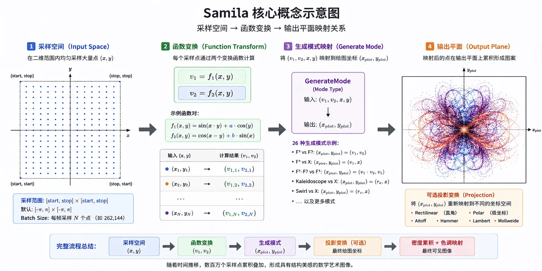
What is Samila?

Samila's core idea is simple yet powerful: scatter sampling points uniformly across a 2D sampling space, compute two output values for each sample point (x, y) via two transform functions f1 and f2, then map these outputs to a scatter coordinate on the plane according to a generate mode. When millions of such scatter points accumulate and overlap, structurally beautiful mathematical patterns emerge.

Unlike iterative dynamical systems such as symmetry chaos or map attractors, Samila does not track particle states — each frame is a completely new independent sampling of the function space. Over time, the accumulation buffer progressively fills all possible screen positions, ultimately revealing the full structure of the function space.

Mathematical Model

Given two transform functions f1(x,y) and f2(x,y), and a sampling range [start, stop]:

Where GenerateMode determines how the four variables (v1, v2, x, y) map to plot coordinates.

Generate Mode Categories

Generate modes are Samila's most creative design element. They decide which data maps to the x-axis and which to the y-axis:

Category	Modes	Description
Function vs Function	F1 vs F2, F2 vs F1	Classic mode showing the relationship between two functions
Function vs Coordinate	F1 vs X, F2 vs X, F1 vs Y, F2 vs Y	Shows how function values vary with input coordinates
Coordinate vs Function	X vs F1, X vs F2, Y vs F1, Y vs F2	Shows how input coordinates influence function output
Function Product	F1·F2 vs F1, F1·F2 vs F2, F1 vs F1·F2, F2 vs F1·F2	Introduces nonlinear coupling for more complex structures
Kaleidoscope	Kaleidoscope vs X, X vs Kaleidoscope	Sector-folded polar coordinates of (v1, v2) producing symmetric patterns
Swirl	Swirl vs X, X vs Swirl	Polar radius distortion producing flowing swirl effects
Warp	Warp vs X, X vs Warp	Sine domain warping producing organic wave structures
Cosine Modulation	CosMod vs X, X vs CosMod	Dual-frequency cosine modulation producing geometric grid textures
Radial Distance	Radial vs X, X vs Radial	Power-law mapping of distance producing radial structures
Fold Tiling	Fold vs X, X vs Fold	Periodic folding producing tiled geometric textures

Map Projections

Projection transforms remap generate-mode output coordinates into new coordinate spaces:

Projection	Description	Best For
Rectilinear	Direct mapping, preserving original coordinates	Showcasing the function's raw structure
Polar	Polar mapping: x = θ, y = r	Producing swirl and radial patterns, especially effective with trigonometric functions
Aitoff	Equal-area pseudo-azimuthal projection	Creating globe-surface visual impressions
Hammer	Hammer-Aitoff equal-area projection	More compact globe projection effects
Lambert	Azimuthal equal-area projection	Producing map-like visual effects
Mollweide	Equal-area pseudocylindrical projection	Producing elegant elliptical boundaries

Tip: When generating random equations, the system automatically recommends the optimal generate mode and projection based on the equation type. Different combinations produce dramatically different visual results — experiment boldly!

Aesthetic Principles of Random Equation Generation

Samila's built-in random equation generator differs from ordinary randomization — it converges based on aesthetic scoring:

1. Function Tiering: Trigonometric functions (sin/cos) are Tier 1 (high aesthetics), because their boundedness and periodicity are the foundation of visual beauty
2. Weighted Selection: sin/cos are 7× more likely to be selected than other functions
3. Mandatory Trig: Both equations must contain at least one trigonometric function
4. Asymmetric Complexity: f1 and f2 maintain different complexity levels, avoiding excessive symmetry leading to monotony
5. Parameter Convergence: Parameter values are controlled within [0.1, 2.5] to ensure manageable graphic density
6. Quality Validation: Randomly samples 8 points to verify the equation won't produce extreme values or constant output

---

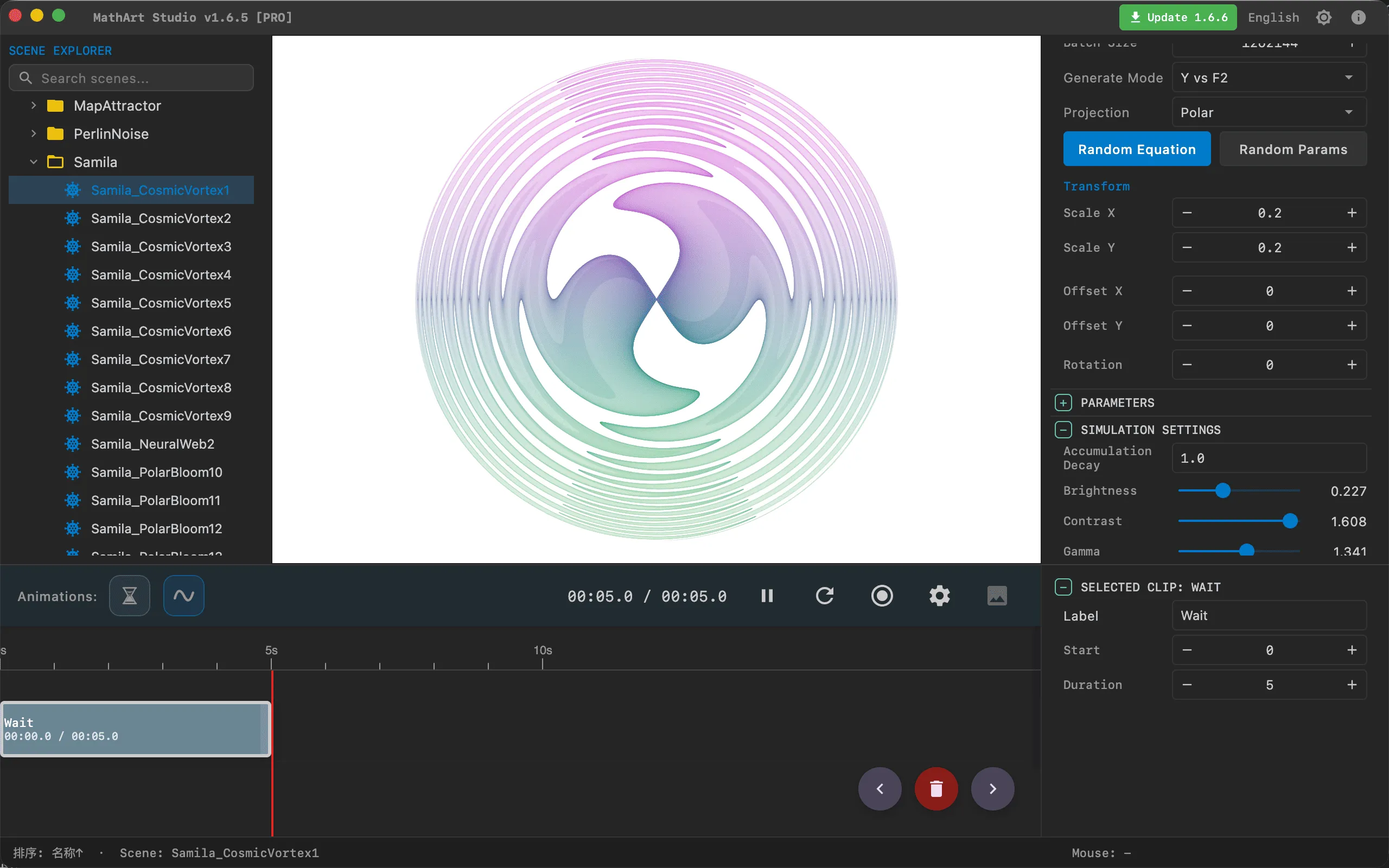
🖥️ Interface Overview

All controls are located in the inspector panel on the right, divided into five main sections:

1. Geometry: Define transform equations, select generate mode and projection, adjust spatial transforms
2. Simulation: Configure sampling parameters, tone mapping, and color speed
3. Formulas: Display mathematical formulas and annotations
4. Appearance: Adjust background color and gradient palette
5. Parameters: Define custom constants used in equations

---

⚙️ Configuration Guide

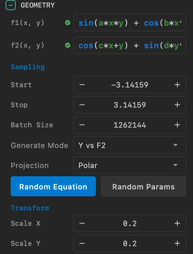
1. Geometry

The geometry panel is Samila's core control area, where you define mathematical equations and spatial mapping rules.

Equation Definition

• f1(x,y): The first transform function, supporting arbitrarily complex mathematical expressions

  • Supported operators: +, -, *, /, ^ (exponentiation)
  • Supported functions: sin, cos, tan, sinh, cosh, tanh, asin, acos, atan, sqrt, abs, log, exp, round, pow
  • Supported variables: x, y (sampling coordinates), and any custom parameter names (a, b, c, d, e, etc.)
  • Default: sin(x*y)

• f2(x,y): The second transform function, with the same syntax as f1

  • Default: cos(x-y)

Usage Tip: Variable and parameter names in equations are case-sensitive. If you define parameter a, you must add the corresponding parameter name and value in the Parameters panel.

Random Equation Button

This is Samila's most delightful feature. Clicking the "Random Equation" button will:

1. Generate a pair of aesthetically pleasing random equations
2. Automatically compute optimal parameter combinations
3. Intelligently recommend the best generate mode and projection
4. Dynamically estimate the output range and set appropriate scale

With a single click, you get a completely different, visually stunning mathematical pattern.

Sampling Range

• Start / Stop: Define the boundaries of the sampling space
  • Default: [-π, π] (from -3.14 to 3.14)
  • Purpose: Sampling points are uniformly distributed within this interval
  • Recommendation: Keep the default [-π, π], as this range is most friendly to trigonometric functions. Expanding the range may reduce the pattern's layered texture

Generate Mode Selection

Choose from the dropdown menu among 26 generate modes spanning function comparison, kaleidoscope, swirl, warp, and other categories. Switching modes instantly transforms the visual output on the canvas.

Projection Selection

Choose a projection from the dropdown menu. Polar projection is most commonly used for swirl-like patterns, while Rectilinear is best for showcasing the function's raw structure.

Spatial Transforms

• Scale X/Y: Adjust the horizontal/vertical scaling of the scatter plot

  • Default values are auto-computed based on the equation
  • Increase Scale to enlarge the pattern (zoom in)
  • Decrease Scale to shrink the pattern (zoom out)

• Offset X/Y: Adjust the position of the scatter plot

  • Effective NDC range: [-1, 1]
  • Positive values move the pattern toward the upper-right of the screen

• Rotation: Rotate the entire scatter plot (in radians)

  • Positive = counterclockwise, Negative = clockwise

Tip: Samila is always 2D rendering — Z-axis scale and offset typically need no adjustment.

---

2. Simulation

Controls sampling behavior and visual presentation. Samila uses a pure GPU rendering pipeline — all computation happens on the GPU.

Sampling Settings

• Batch Size: Number of points sampled per frame

  • Default: 262,144 (~260K)
  • Purpose: Determines the sampling density per frame in the sampling space
  • Recommendations:
    • Fast preview: 100,000 – 200,000
    • Fine rendering: 300,000 – 500,000
    • High-res output: 500,000+
  • Note: Excessively large batch sizes consume more GPU memory

• Alpha: Transparency of each sample point

  • Range: 0.0 – 1.0
  • Default: 0.1
  • Purpose: Smaller Alpha produces smoother density transitions; larger Alpha produces more distinct points

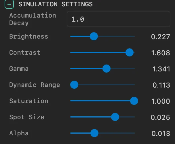
Tone Mapping

Tone mapping is the critical step that converts accumulated floating-point density data in the GPU into visible colors on screen:

• Brightness: Overall brightness offset

  • Range: 0.0 – 1.0
  • Default: 0.5
  • Purpose: Increase when the image is too dark, decrease when too bright

• Contrast: Contrast of the density distribution

  • Range: 0.1 – 2.0
  • Default: 1.0
  • Purpose: Higher contrast makes bright areas brighter and dark areas darker

• Gamma: Nonlinear brightness mapping

  • Range: 0.1 – 10.0
  • Default: 2.2
  • Purpose: Controls mid-tone brightness. 2.2 is the standard sRGB gamma value

• Dynamic Range: Density mapping range

  • Range: 0.1 – 1.0
  • Default: 0.5
  • Purpose: Larger values preserve more shadow detail; smaller values make the image brighter

• Saturation: Color vividness

  • Range: 0.0 – 1.0
  • Default: 0.8
  • Purpose: 0.0 = grayscale, 1.0 = full saturation

Color Settings

• Color Speed: Controls how quickly colors change across the output space

  • Default: 0.22
  • Purpose: Affects the hue distribution density of the palette across the image

• Color Phase: Offset phase of the palette

  • Default: 180.0
  • Purpose: Rotates the palette's starting position

Trail Effect

• Show Trails: Enable the trail effect

  • Enabled by default
  • Purpose: When enabled, old density data gradually decays over time, producing a dynamic trail effect

• Trail Lifetime: Trail duration in seconds

  • Default: 4.0 seconds
  • Purpose: Controls the time for old density data to decay to 1%. Smaller values cause trails to fade faster

• Accumulation Decay: Extra decay coefficient

  • Range: 0.0 – 1.0
  • Default: 1.0 (no extra decay)
  • Purpose: Values below 1.0 apply additional decay, creating a fade-out effect

---

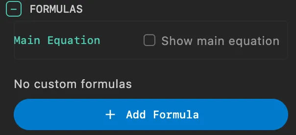
3. Formulas

Display mathematical formulas and equations in the scene.

Main Equation Display

• Show Main Equation: Toggle main equation display on/off

  • Purpose: Displays the current f1 and f2 transform equations in the scene
  • Auto-generated: The system automatically generates LaTeX formulas from the current equations

• Main Equation Position & Style:

  • X: Horizontal position coordinate
  • Y: Vertical position coordinate
  • Scale: Formula scale factor
  • Color: Formula color

Custom Formulas

Add multiple custom formulas to the scene:

• Add Formula: Click "Add Formula" to add a new formula
• Formula Content:
  • LaTeX: LaTeX-formatted mathematical expression
  • X / Y: Display position
  • Scale: Scale factor
  • Color: Formula color
• Delete Formula: Click the delete button in the formula's top-right corner to remove

---

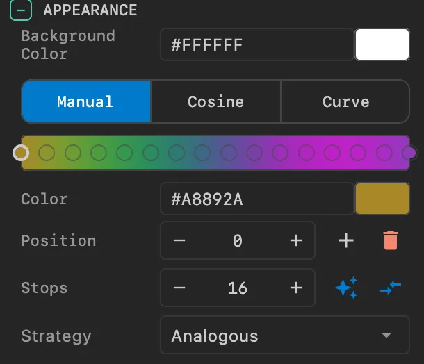
4. Appearance

Background Color

• Background Color: Set the rendering background color
  • Dark backgrounds typically better highlight the scatter plot's color layering
  • Black is the classic choice

Gradient Palette

Samila uses a 1D LUT (Look-Up Table) texture for coloring, supporting three gradient modes:

• Manual Mode:

  • Manually add, delete, and adjust color stops
  • Drag to reorder colors
  • Four random strategies: Monochromatic, Analogous, Complementary, Split Complementary

• Cosine Mode:

  • Uses the IQ cosine palette formula: color(t) = a + b · cos(2π(c·t + d))
  • Separately control offset, amplitude, frequency, and phase for R/G/B channels
  • One-click randomization and application

• Curve Mode:

  • Editable Bézier curves for R/G/B channels independently
  • Offers the most flexible color control
  • One-click randomization and application

Palette Switch Tip: Switching palette modes triggers an accumulation buffer rebuild. The image smoothly transitions to the new colors within approximately 0.5 seconds.

---

5. Parameters

Manage custom parameters used in equations.

• Add Parameter: Enter a parameter name (e.g., a) and value (e.g., 1.5) in the bottom input fields, then click the add button
• Edit Parameter: Use the slider or directly type a value to modify parameters in real time
• Delete Parameter: Click the delete button on the right side of a parameter row to remove it

Important: Modifying equation structure (adding/removing parameter names) requires shader recompilation and may cause a brief stutter. Modifying parameter values does not require recompilation and can be hot-updated in real time.

---

🎬 Animation and Timeline

Parameter Oscillation Animation

Samila supports Parameter Oscillation Animation, which makes parameters oscillate sinusoidally within a specified range.

How It Works

1. Specify the oscillation step, range (min, max) for each parameter
2. Parameter values oscillate sinusoidally within [min, max]: value = mid + amp · sin(phase)
3. Oscillation speed is controlled by the step value

Persistent Parameter Drift

When the parameter animation finishes, the oscillation doesn't stop immediately — the system enters persistent drift mode, where parameters continue oscillating at full speed until a stop command is received. This means the pattern continues to dynamically evolve during the animation's wait phase.

Animatable Parameters

All custom parameters in equations (a, b, c, d, e, etc.) support animation.

Camera Animation

Samila also supports standard camera animation:

• Rotation: Rotate the camera around the pattern
• Alignment: Align the camera to a specific angle
• Zoom: Adjust camera distance

Configuration Method

Define animation sequences through the timeline array in JSON configuration files:

{
  "timeline": [
    {
      "type": "animate",
      "duration": 15.0,
      "easing": "SINE_IN_OUT",
      "actions": [
        {"method": "rotateTheta", "args": [6.283]}
      ]
    },
    {
      "type": "hold",
      "duration": 2.0
    }
  ]
}

Parameter animation configuration example:

{
  "timeline": [
    {
      "type": "animate",
      "duration": 8.0,
      "easing": "LINEAR",
      "actions": [
        {
          "method": "paramStart",
          "args": [{
            "parameters": {
              "a": {"enable": true, "step": 0.002, "min": 0.5, "max": 2.5},
              "b": {"enable": true, "step": 0.003, "min": 0.8, "max": 2.0}
            }
          }]
        }
      ]
    },
    {
      "type": "hold",
      "duration": 10.0
    },
    {
      "type": "animate",
      "duration": 2.0,
      "easing": "SINE_IN_OUT",
      "actions": [
        {"method": "paramStop", "args": [{}]}
      ]
    }
  ]
}

---

🚀 Performance & Best Practices

Recommended Configurations

Goal	Batch Size	Alpha	Gamma	Dynamic Range	Dot Size
Fast Preview	50K – 100K	0.2 – 0.5	2.2	0.5	0.02 – 0.05
Real-time Interaction	200K – 300K	0.1 – 0.2	2.2	0.4 – 0.6	0.01 – 0.02
High-Quality Image	500K+	0.05 – 0.1	2.2	0.3 – 0.5	0.005 – 0.01

Performance Optimization Tips

1. Batch Size Adjustment:

   • Reducing Batch Size is the most direct way to optimize performance
   • For high-complexity projections like Mollweide, use smaller Batch Size

2. Dot Size & Alpha:

   • Smaller Dot Size with smaller Alpha produces the finest detail
   • Larger Dot Size reduces the number of frames needed to reach visual saturation

3. Tone Mapping Tuning:

   • With smaller Batch Size, slightly lower Dynamic Range to brighten the image
   • Gamma has a significant impact on visual appearance — 2.2 is the best starting point

4. Use Random Equations:

   • If you're not mathematically inclined, the random equation button is the fastest way to get started
   • Once you find a pattern you like, fine-tune parameters for personalized optimization

---

❓ FAQ

Image is completely black or too dark

Problem: The rendered result is nearly black

Cause: Insufficient density accumulation or inappropriate tone mapping parameters

Solutions:

• Increase Batch Size (e.g., from 260K to 500K)
• Increase Brightness (e.g., from 0.5 to 0.8)
• Decrease Dynamic Range (e.g., from 0.5 to 0.3)
• Decrease Gamma (e.g., from 2.2 to 1.5)
• Wait a few seconds for density to accumulate sufficiently

Image is completely white

Problem: The rendered result is entirely white

Cause: Tone mapping parameters make density excessively bright

Solutions:

• Decrease Brightness
• Increase Dynamic Range
• Increase Dot Size while decreasing Alpha

Pattern looks unstructured

Problem: The scatter plot looks like random noise

Cause: Equation lacks periodicity or distribution is too uniform

Solutions:

• Use the random equation button to get a structured starting equation
• Try switching generate modes, especially F1 vs F2 or Polar projection
• Ensure equations contain trigonometric functions (sin/cos)

Flickering after parameter changes

Problem: Brief flickering or clearing after modifying parameter values

Cause: Parameter changes trigger accumulation buffer rebuild (this is normal behavior)

Solutions:

• The accumulation buffer refills within approximately 0.5–1.0 seconds
• This is necessary to ensure the image is fully consistent with the current parameters

No effect after modifying equations

Problem: No visual change after modifying f1 or f2 equations

Cause: Equation modifications require clicking "Apply" to compile the new shader

Solutions:

• Click the "Apply" button at the top of the Inspector panel after modifying equations
• Verify correct equation syntax — no mismatched parentheses, etc.

---

📐 Classic Examples

Polar Kaleidoscope Pattern

f1: sin(a*x*y) + cos(b*x)
f2: cos(c*x+y) + sin(d*y)
Generate Mode: Kaleidoscope vs X
Projection: Polar
Parameters: a=2.0, b=1.0, c=1.5, d=0.5

Swirl Flow Effect

f1: sin(a*x*y) + cos(b*x)
f2: cos(c*x+y) + sin(d*y)
Generate Mode: Swirl vs X
Projection: Polar
Parameters: a=2.0, b=1.0, c=1.5, d=0.5

Hammer Projection Effect

f1: sin(a*x*y) + cos(b*x)
f2: cos(c*x+y) + sin(d*y)
Generate Mode: F1 vs F2
Projection: Hammer
Parameters: a=2.0, b=1.0, c=1.5, d=0.5

---

🔧 Technical Details

GPU Rendering Pipeline

Samila uses a random sampling + density accumulation GPU pipeline (distinct from iterative particle systems):

1. Splat Pass:

   • Vertex Shader endogenously generates random sample positions via PCG Hash algorithm
   • No CPU VBO upload needed — drastically reduces CPU→GPU bandwidth consumption
   • Computes f1 and f2 for each sample point, then applies generate mode and projection
   • Projects particles onto accumulation buffer using GL_POINTS + additive blending (GL_ONE, GL_ONE)

2. Decay Pass:

   • Copies the previous frame's accumulation buffer to the current write buffer with the decay factor
   • Simultaneously applies density ceiling constraint (default: 300) to prevent indefinite high-density accumulation

3. Present Pass:

   • Applies logarithmic tone mapping to accumulated density: value = log(density) → brightness
   • Executes the complete tone mapping chain: brightness → contrast → gamma → dynamic range → saturation
   • Uses Palette LUT for spatially-driven color mapping

PCG Hash Random Sampling

One of Samila's core innovations: the vertex shader endogenously generates random sample positions through gl_VertexID ^ u_frameSeed via the PCG Hash algorithm, requiring no CPU precomputation or VBO upload. The per-frame changing random seed ensures frame-to-frame randomness while maintaining efficiency and independence.

Noise-Driven Palette

Samila computes Simplex 2D noise in the Vertex Shader to drive the palette's U coordinate. Since all fragments in a GL_POINT share the same varying values, the noise computation executes only once per vertex (rather than being repeated per fragment), significantly saving GPU compute resources.

Adaptive Tone Mapping Scale

Samila's tone mapping system automatically adapts to different rendering scenarios:

• Non-decay mode: Uses a √N growth formula to prevent density from infinitely increasing over time
• Decay mode (trails enabled): Computes per-frame decay coefficient from trail lifetime, automatically matching steady-state density to a reasonable brightness range
• Ceiling constraint: The density ceiling provides an upper bound for scale computation, ensuring the brightest pixels never overexpose

---

🎨 Creative Tips

Exploration Strategy

1. Start with random equations: The random equation button is the fastest way to get started
2. Switch generate modes and projections: The same equation produces dramatically different results under different mode/projection combinations
3. Fine-tune parameters: Change individual parameter values to observe continuous pattern evolution
4. Try custom equations: Once familiar with basic patterns, write your own mathematical expressions

Visual Tuning

1. Tone Mapping:

   • First adjust Dynamic Range to make the pattern overall visible
   • Then adjust Gamma to reveal mid-tone details
   • Finally fine-tune Brightness and Contrast

2. Color Schemes:

   • Use cosine palette mode to quickly generate harmonious color schemes
   • Dark backgrounds with high saturation colors typically produce the best results
   • Adjust Color Speed and Color Phase to change color distribution density

3. Dot Size & Alpha:

   • Small dots + low alpha = extreme smoothness and refinement (best for final output)
   • Large dots + high alpha = quick pattern structure preview (best for exploration phase)

Animation Design

1. Parameter Oscillation:

   • Set different oscillation speeds for different parameters to create rich dynamic variation
   • Use persistent drift to keep the pattern evolving during the wait phase

2. Camera Movement:

   • Rotation animation is the simplest and most effective animation form
   • Note: in animation scenarios, each frame executes 6 splat passes to compensate for the inability to accumulate density across frames

---

⚠️ Important Notes

1. Equation Syntax:

   • Multiplication must be explicitly written as * (a*x, not ax)
   • Use pow function or ^ symbol for exponentiation
   • Parameter names are case-sensitive

2. GPU Memory:

   • Excessively large Batch Size consumes more GPU memory
   • Accumulation texture size equals viewport resolution, using RGBA32F format

3. Accumulation Buffer Rebuild:

   • Modifying parameter values, equations, or palette triggers accumulation buffer rebuild
   • Visual density takes approximately 0.5–1.0 seconds to recover during rebuild
   • This is normal behavior, ensuring the image is always consistent with current parameters

4. Animation Performance:

   • In animation scenarios (parameter changes or rotation), each frame executes 6 splat passes as compensation
   • Use smaller Batch Size during animation to maintain smoothness

5. Parameter Drift:

   • After parameter animation ends, parameters continue changing in drift mode
   • Drift only stops upon explicit paramStop call

---

📚 Reference Resources

Inspiration

• Samila Mappings — samila mappings
• Generative Art: A Practical Guide Using Processing — A classic introduction to generative art

Mathematical References

• Wikipedia: Map Projection — Mathematical principles of map projections
• IQ's Cosine Palette — Detailed explanation of cosine palette formula

Software Documentation

• OpenGL Shader Programming Guide
• GLSL Language Specification